Explainability In Machine Learning: Top Techniques

Explaining Explainable AI

In the area of machine learning, models are used to make complex predictions and decisions. These advanced models generate incredible findings for a variety of domains, however, they have been nicknamed “black boxes” due to the opaque nature of their internal workings. It is therefore incredibly difficult for an engineer to trace back the root cause of a prediction, which is where ML explainability methods and technologies come into play.

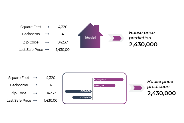
In the case of predicting house prices based on a set of features, explainability triages and normalizes the importance of various features (square feet, number of bedrooms, zip code, last sale price, etc.) to a prediction of a home sales price.

What Are the Different Techniques for ML Explainability?

There are different approaches for explainability that teams might use based upon the use case and environment. These are normally driven by:

• Model Type: neural network, tree, image-based, or language-based
• Whether or not your team has direct access to the model
• The speed versus accuracy trade-off
• Computational costs
• Global and local feature importance
• AI governance, risk management and compliance needs

TL;DR: explainability is a tool in the toolbox that helps teams understand the decisions made by their models and the impact those decisions have on their customers/users as well as their company’s bottom line. It is an approximation in itself, and there is no “perfect” explainer — each methodology has a trade-off.

After a quick overview of SHAP and LIME, we’ll focus on model-specific and model-agonistic explainability techniques.

What Is SHAP?

SHAP (Shapley Additive exPlanations) is a method used to break down individual predictions of a complex model. The purpose of SHAP is to compute the contribution of each feature to the prediction in order to identify the impact of each input. The SHAP explanation technique uses principles rooted in cooperative coalitional game theory to compute Shapley values. Much like how cooperative game theory originally looked to identify how the cooperation between groups of players (“coalitions”) contributed to the gain of the coalition overall, the same technique is used in ML to calculate how features contribute to the model’s outcome. In game theory, certain players contribute more to the outcome and in machine learning certain features contribute more to the model’s prediction and therefore have a higher feature importance.

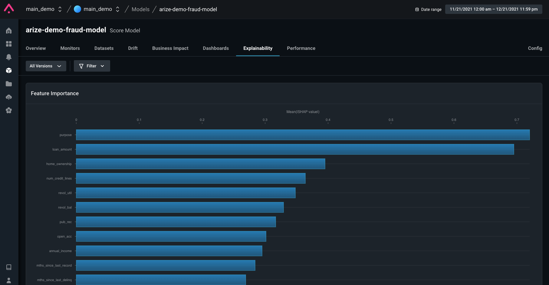
In the field of AI, these complex models benefit greatly from a proven method that is able to provide predictions for nonlinear models. The Shapley value is the average of all the marginal contributions to all possible coalitions. A data instance’s feature values operate as coalition members. The Shapley value explanation is expressed in the form of an additive approach to attribute a linear model. SHAP values not only reveal feature relevance but also whether the feature has a positive or negative influence on predictions. In the example of a fraud model below, the features “purpose” and “loan amount” disproportionately help determine whether the model predicts fraud.

It’s worth noting that the Kernel-based SHAP also does perturbations but these are based on background or reference datasets. A linear model is built to extract the Shapley values based on the perturbations.

What is LIME?

LIME, or Local Interpretable Model-Agnostic Explanations, is a technique that provides  local ML explainability by approximating “black boxes” with an interpretable model for each prediction. These local models are created from understanding how perturbations in a model’s inputs affect the end-prediction of the model.

LIME attempts to understand the relationship between a particular example’s features and the model’s prediction by training a more explainable model such as a linear model with examples derived from small changes to the original input. At the end of training, the explanation can be found from the features for which the linear model learned coefficients above particular thresholds (after accounting for some normalization). The intuition behind this is that the linear model found these features to be most important in explaining the model’s prediction, and therefore for this local example you can reason about the contributions that each feature made in explaining the prediction that your model made.

Let’s imagine you have a black-box model where you only have access to the inference data and the corresponding model predictions, but not the initial training data. LIME creates a new dataset consisting of the perturbed samples and their corresponding black-box model predictions.

On this new dataset, LIME trains an interpretable model weighted by the proximity of the sampled instances to the instances of interest. A trainable model should be a good approximation to machine learning model predictions locally, but not necessarily a good global fit.

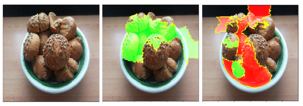
LIME can be used for tabular, image, or text datasets. The below example of a bowl of bread has LIME explanations for the top two classes (bagel, strawberry) for image classifications made by Google’s Inception V3 neural network. The prediction and explanation for “bagel” are very reasonable, even if the prediction is wrong – there are clearly no bagels since the hole in the middle is missing.

Selecting SHAP or LIME: Feature Importance Vs. Attribution of Value

The SHAP approach to explainability is designed to attribute an outcome — say, a prediction of house price — to a measured combination of features. We consider this a statistical attribution of a model’s output to a set of inputs. For example, the house’s 4,100 ft2 contributed to $1.1 million of the total house price prediction of $2.43 million.

The LIME approach generates a set of feature importances but does not tie those feature importances to exact attributions of the model output. For example, LIME can’t tell you the exact dollar amount that the contributed square footage made to the predicted housing price but it can tell you the most important feature or features to that prediction.

TL;DR: ML teams in industry often use both SHAP and LIME, but they use LIME to get a better explanation of a single prediction and SHAP to understand the entire model as well as feature dependencies.  

In terms of computational time and cost, LIME is faster than SHAP. However, while Shapley values take a long time to compute, SHAP makes it possible to compute the many Shapley values needed for global model interpretations. LIME can still be useful with tabular, text, and image data — especially if the model is trained using uninterpreted functions. That said, since LIME approximates these models with a more interpretable model, there is a tradeoff between the complexity of LIME and the trustworthiness of LIME.

Model Type-Agnostic & Model Type-Specific Explainability Approaches

Model-specific methods work by exploring and accessing the interior of the model, such as interpretation of regression coefficient weights or P-values ​​in a linear model, or counting the number of times a feature is used in an ensemble tree model.

The model-agnostic method investigates the relationships between I/O pairs of trained models. They do not depend on the internal structure of the model. These methods are useful when there is no theory or other mechanism to interpret what is happening in the model.

Model Type Specific

What is TreeSHAP?

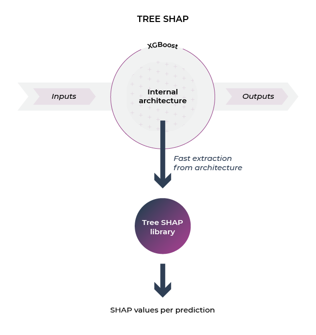
TreeSHAP is a fast explainer used for analyzing decision tree models in the Shap python library. TreeSHAP is designed for tree-based machine learning models such as decision trees, random forests and gradient boosted trees. TreeSHAP is offered as a rapid, model-specific alternative to KernelSHAP; however, it can sometimes produce unintuitive feature attributions.

Given the prevalence of XGBoost, TreeSHAP is an explainer approach heavily used in various teams. The tree explainer makes use of the structure of the tree algorithm to extract and generate SHAP values much faster than the Kernel explainer.

TL;DR: TreeSHAP is a great fast explainer if you have XGBoost or LightGBM.

TreeSHAP calculates in polynomial time, not exponential time. The basic idea is to move all possible subsets down the tree at the same time. To calculate the single-tree forecast, you need to track the number of subsets in each decision node. This depends on the subset of parent nodes and the split function.

Neural Networks: Deep Explainer

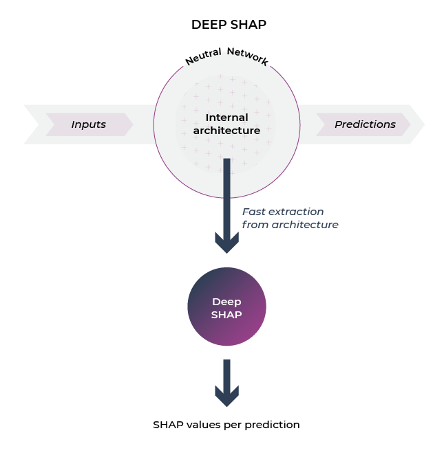
The figure above depicts the working of the DeepExplainer (DEEP SHAP).

TL;DR: Deep explainer (deep SHAP) is an explainability technique that can be used for models with a neural network based architecture. This is the fastest neural network explainability approach and is based on running a SHAP-based version of the original deep lift algorithm. 

A popular way to leverage SHAP values to explain predictions of deep learning models (neural networks) is with the method DeepExplainer. DeepExplainer runs on deep learning frameworks to add explainability to neural network models by using DeepLIFT and Shapley values. DeepExplainer is an enhanced version of the DeepLIFT (Deep Learning Important FeaTures), a method for decomposing the output prediction of a neural network on a specific input by backpropagating the contributions of all neurons in the network to every feature of the input.

Lundberg and Lee, NIPS 2017, showed that the per node attribution rules in DeepLIFT can be chosen to approximate Shapley values. By integrating over many background samples, DeepExplainer (deep SHAP) estimates approximate SHAP values such that they sum up to the difference between the expected model output on the passed background samples and the current model output (f(x) – E[f(x)]).

Neural Networks: Expected Gradients and Integrated Gradients

Expected and integrated gradients are both explainability techniques that can be used with neural network models.

TL;DR: expected gradients are a fast explainability technique useful for differentiable models; it offers different approximations than deep explainer and is slower than deep explainer. Integrated ingredients is an older local method that helps account for each individual prediction. 

Expected gradients are a fast explainability technique useful for differentiable models. You can think of expected gradients as a SHAP-based version of integrated gradients, an older explainability technique. It extends the Shapley game-theory approach to integrated gradients so the outputs of the feature attributions sum to the output.

Integrated gradients are a technique for attributing the predictions of a classification model to input features. It can be used to visualize the relationship between input features and model predictions. It is a local method that helps account for each individual prediction. For example, in the Fashion MNIST dataset, if we take the image of a shoe, then the positive attributions are the pixels of the image which make a positive influence on the model classifying the image as a  shoe. The integrated gradient method is mainly used to identify errors in the model, where corrections can be made to improve the accuracy of the model.

Linear Regression: Linear SHAP

Linear SHAP is an explainability approach designed for linear regression models. It’s model-specific and fast.

A linear regression model predicts a target as a weighted sum of its inputs. The linearity of the learned relationship facilitates interpretation. Linear regression models have long been used by statisticians, computer scientists, and others involved in quantitative problems.

Model Type Agnostic

What is Kernel SHAP?

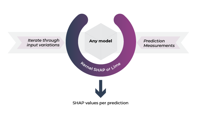
Kernel SHAP is a slow, perturbation-based Shapley approach that theoretically works for all types of models but is rarely used by teams in the wild (at least in production).

TL;DR: Kernel SHAP tends to be way too slow to be used in practice extensively on anything but small data. It also tends to cause confusion among teams. When teams complain about SHAP being slow, usually it’s because they tested Kernel SHAP.

Kernel SHAP works by calculating the contributions of each feature value to the prediction for an instance “x.” Kernel SHAP is made up of five steps: examine coalitions, obtain a prediction for each coalition, calculate the weight for each using kernel SHAP, create a weighted linear model and return the Shapley values “k,” the linear model’s coefficients.

What is a Surrogate Model?

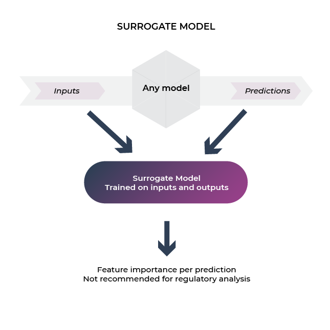
Surrogate model is an explainability approach designed to build a transparent model off of the predictions of an actual model. The model is built in parallel with the model data. It is used when an outcome of interest cannot be easily directly measured, so a model of the outcome is used instead.

TL;DR: Surrogate model is useful if you don’t have the original model to extract SHAP; you can build a surrogate off of model decisions. It’s less ideal for regulatory use-cases as it is highly dependent on the data the model sees.

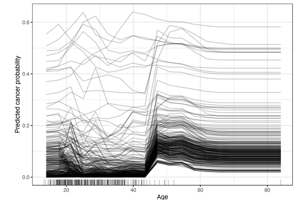
What is Individual Conditional Expectation (ICE)?

Individual conditional explanation (ICE) plots visualize one line per instance to show how the instance’s prediction changes when a feature changes.

Though ICE curves can uncover heterogeneous relationships, the ICE curve requires the two features to be drawn on multiple overlapping surfaces, which can be hard to read.

Conclusion

Explainability is a growing field gaining popularity, with ongoing research. As you explore different explainability methods, hopefully this primer is helpful.