Integrated gradients are a technique for attributing the predictions of a classification model to input features. It can be used to visualize the relationship between input features and model predictions. It is a local method that helps account for each individual prediction. For example, in the Fashion MNIST dataset, if we take the image of a shoe, then the positive attributions are the pixels of the image which make a positive influence on the model classifying the image as a shoe. The integrated gradient method is mainly used to identify errors in the model, where corrections can be made to improve the accuracy of the model. Engineers reach for it when they need feature-level credit assignments that satisfy basic sanity checks better than raw gradients alone.
Build better agents with Arize
Trace, evaluate, and learn. Build agents that work with Arize AX and start tracing your runs today.
Prefer open source? Try Arize Phoenix for self-hosted, open source agent observability.
Key takeaways
- Integrated gradients integrate the gradient along a straight path from a baseline input to the actual input, multiplying by the input difference to produce attributions.
- Attributions approximate how much each feature moved the logit or score relative to a chosen baseline.
- Baseline choice is the largest practical decision; bad baselines produce misleading heatmaps even when code is correct.
- The method applies to differentiable models and works on images, text embeddings, and tabular tensors alike.
- Use attributions to debug misclassifications, not as a standalone fairness audit without domain review.
Mathematical sketch
Let x be the input vector, x’ a baseline, and F the model output for the target class (or scalar score). Integrated gradients define the attribution for feature i as:
IG_i(x) = (x_i – x’_i) * integral from 0 to 1 of dF(x’ + alpha*(x – x’)) / d(x_i) d alpha
In words: walk along a straight line from baseline to input, record how the gradient with respect to feature i changes, average that gradient over the path, and scale by the feature delta. Summing attributions across features equals F(x) – F(x’) under typical smoothness assumptions, which is the completeness property practitioners expect from additive explanations.
Implementation uses Riemann sums: pick steps along alpha, compute gradients at interpolated inputs, accumulate, and multiply by (x – x’).
Why not plain gradients?
Vanilla gradients at the input can saturate: if the model is flat near x, gradients vanish even when features matter elsewhere on the path. Integrated gradients aggregate gradient information along the entire path from baseline to input, reducing saturation artifacts that plague single-point gradient saliency maps.
They also align better with axioms such as sensitivity: if a feature differs from baseline and changes the output, it receives non-zero attribution. Implementation still requires thoughtful baselines.
Choosing a baseline
The baseline x’ should represent “absence” of signal in a way the model understands. For images, a black or blurred image is common. For text, a padding or mask token embedding baseline appears in many notebooks. For tabular data, mean or median feature vectors are typical.
A weak baseline makes attributions hard to interpret. If the baseline is already predictive, path integrals shrink. Domain experts should sign off on baseline semantics for high-stakes models.
Local explainability in practice
Integrated gradients explain one prediction at a time. Heatmaps over images highlight pixels that pushed toward the predicted class. For text, attributions land on token embeddings or input dimensions after backprop through the embedding layer.
Compare attributions on correct versus incorrect examples. Spurious correlations often show up as large attributions on background textures, timestamps, or watermark pixels. Once located, teams can augment data, adjust training, or add constraints.
The Fashion MNIST shoe example from the original definition illustrates the pattern: pixels along the sole and upper receive positive attribution for the shoe class, while background pixels stay near zero when the model behaves well.
Global views and cohort analysis
Local maps do not automatically summarize model behavior. Aggregate absolute attributions across a validation slice to see global feature importance trends, or condition on subgroups to compare cohorts. Those aggregates are descriptive statistics, not causal effects.
Pair integrated gradients with performance slices. If accuracy drops on a demographic cohort, attribution differences on that cohort may reveal over-reliance on proxy features.
Limitations
Compute cost. Each step requires a backward pass. High-resolution images and long sequences need step count tuning.
Baseline dependence. Different baselines yield different maps; document the choice in reports.
Not causal. Attributions show correlation along an integration path, not intervention effects in the real world.
Adversarial sensitivity. Small input perturbations can change gradients sharply; treat maps as debugging hints.
Other methods such as SHAP or LIME offer different tradeoffs. Integrated gradients target differentiable models and integrate path gradients rather than fitting a local linear surrogate.
Ties to monitoring and shipping
Attribution drift can precede accuracy drift: the model still predicts but for the wrong reasons. After retraining or fine-tuning, spot-check attributions on a golden set. Concept and data drift monitoring catches input shifts; attribution checks catch internal reasoning shifts on fixed inputs.
Before shipping vision models, run integrated gradients on validation failures to catch label noise and spurious backgrounds. Shipping image classification with confidence emphasizes validation discipline that pairs naturally with local explainability reviews.
Model lifecycle management should store explanation configs (baseline, steps, target layer) next to model versions so comparisons across releases stay apples to apples.
FAQ
How many integration steps do I need?
Start with 20 to 50 steps for images and increase if attributions look noisy. Measure stability: if maps change materially between 32 and 64 steps, keep the higher count for reporting.
Can I use integrated gradients for regression?
Yes. Set F to the scalar regression output or to a logit if you analyze a classification head. Completeness holds for the chosen scalar output.
How do integrated gradients compare to SHAP?
Both provide additive feature attributions under different constructions. Integrated gradients use a path integral from a baseline; SHAP uses Shapley values from cooperative game theory. They can disagree; pick one method per workflow and stay consistent.
Do attributions work on transformer models?
Yes, with backprop through embeddings. Token-level heatmaps require attributions on embedding dimensions or use specialized tools that map gradients to tokens. Watch memory on long contexts.
Should I show attributions to end users?
Usually not without review. They are valuable for engineers and reviewers debugging failures. User-facing explanations need simpler language and human validation so heatmaps do not over-promise interpretability.