
Population Stability Index (PSI) measures how much a variable’s distribution has shifted between two samples, usually a reference window (expected) and a current window (actual). PSI compares binned proportions: for each bin, compute the difference in percentage points between actual and expected, multiply by the natural log of their ratio, and sum across bins. Larger PSI means less overlap between distributions, which supports threshold alerts on drift in score and feature monitors.
Credit risk and marketing analytics teams popularized PSI for score stability reports. ML engineers reuse it for feature drift when distributions should stay stable after deployment. PSI is only as trustworthy as your bin definitions and sample sizes.
Build better agents with Arize
Trace, evaluate, and learn. Build agents that work with Arize AX and start tracing your runs today.
Prefer open source? Try Arize Phoenix for self-hosted, open source agent observability.

Key takeaways
- PSI sums over bins: (Actual% − Expected%) × ln(Actual% / Expected%).
- Higher PSI indicates greater distributional shift between reference and comparison samples.
- PSI works for numeric features (via bins) and categorical features (category bins).
- Common rule-of-thumb bands (under 0.1 stable, 0.1 to 0.25 moderate, above 0.25 large) are starting points, not universal law.
- PSI is symmetric in role assignment unlike KL divergence, but bin choices still dominate interpretation.
PSI formula and intuition
Split the reference sample into bins with fixed edges or quantiles. Compute the percentage of rows in each bin for the reference (Expected%) and for the current sample (Actual%). For each bin i:
PSI contribution = (Actual% − Expected%) × ln(Actual% / Expected%)
Total PSI is the sum across bins. When Actual and Expected match in every bin, PSI is zero. When mass moves heavily into bins that were rare in reference, PSI grows.
The log ratio penalizes proportional changes: doubling share in a bin matters more when the reference share was small, but zero counts require smoothing. Add a small epsilon to bin proportions before logs so empty bins do not break the calculation.
Binning choices that make or break PSI
PSI is not a property of raw data alone; it is a property of binned distributions.
Common patterns:
- Equal-width bins on scores bounded [0, 1], such as credit scores or predicted probabilities.
- Quantile bins from reference so each bin holds similar mass, then apply the same edges to current data.
- Category bins for low-cardinality strings; collapse rare levels into an “other” bucket to avoid noisy bins.
Too few bins hide real shifts; too many bins leave sparse counts that inflate PSI from sampling noise. For monthly monitoring, keep bin definitions stable across months so PSI trends are comparable.
Document bin edges in the model artifact. Recomputing PSI after silently changing bins invalidates historical thresholds.
Interpreting PSI magnitude
Practitioners often cite informal bands:
- Below 0.1: little shift; often no action beyond routine logging.
- 0.1 to 0.25: moderate shift; investigate covariates and model performance on recent labels.
- Above 0.25: large shift; treat as significant drift signal, revalidate model or retrain features.
These cutoffs are heuristics from scorecard monitoring, not guarantees for every domain. A PSI of 0.15 on a critical feature may matter more than 0.3 on a decorative one. Tune thresholds using historical incidents and false alert tolerance.
Always inspect which bins moved, not only the scalar PSI. A stable headline PSI can hide offsetting shifts in opposite tails.
PSI vs KL divergence and related metrics
PSI and Kullback-Leibler divergence both compare distributions and appear in drift tooling. Differences that matter in ops:
- Symmetry: PSI swaps cleanly when you label reference vs current either way if you recompute both percentage columns consistently. KL is asymmetric: KL(P || Q) differs from KL(Q || P).
- Scale: PSI is built for decile-style reporting; KL is information-theoretic and unbounded without care.
- Binning: PSI assumes histograms; KL often runs on the same binned vectors in monitoring stacks but can be defined on continuous estimates too.
Use PSI when stakeholders expect scorecard-style stability language. Pair it with performance slices when model, concept, and data drift workflows trigger review.
PSI in ML monitoring workflows
Typical pipeline:
- Freeze a reference window (training, validation, or first production month).
- On each schedule tick, histogram current production with the same bin edges.
- Compute PSI per feature and for model scores.
- Alert above threshold, attach bin-level diff charts, and link to label eval if available.
PSI on model outputs catches scoring drift even when individual features look stable (interaction shifts). PSI on inputs catches upstream pipeline bugs, broken encoders, or real population change.
Integrate alerts into AI model lifecycle management so drift tickets include model version, data window, and bin spec. Promote or rollback based on joint PSI and accuracy trends, not PSI alone.
For NLP classifiers, PSI on embedding clusters or token length buckets complements token-level checks. See NLP sentiment classification monitoring for patterns where label shift and input drift interact.
Failure modes and caveats
- Small samples: sparse bins produce unstable PSI; enforce minimum counts per bin.
- New categories: unseen labels belong in an explicit bin; otherwise PSI misreports as mass shift.
- Leaky re-binning: recomputing quantile edges on current data each week hides slow drift.
- Offsetting shifts: two bins move in opposite directions and partially cancel in the sum.
PSI detects distribution change, not whether performance dropped. Follow up with labeled eval when PSI fires.
FAQ
What is a good PSI threshold for alerts?
Start near 0.1 for sensitive features and 0.25 for exploratory alerts, then calibrate false positive rate on historical data. Domain standards (especially credit scorecards) may mandate specific cutoffs; ML teams should align with compliance when applicable.
Can PSI handle numeric and categorical features?
Yes. Numeric features require binning first. Categorical features use category proportions as bins. High-cardinality fields need bucketing strategy.
Does PSI replace accuracy monitoring?
No. PSI flags input or score distribution change. Accuracy, precision, and recall need labels. Use PSI as an early warning, then validate outcomes.
Why do Actual% and Expected% need smoothing?
If either proportion is zero, the log term is undefined. Add a tiny epsilon or use a Laplace smoothing rule so bins never have literal zero mass in the calculation.
How is PSI different from KS drift tests?
Kolmogorov-Smirnov compares cumulative distributions on sorted continuous values without fixed bins. PSI is bin-based and aligns with decile reporting. KS avoids bin width choices; PSI aligns with business bucket language. Many teams run both.