Wasserstein distance measures how far apart two probability distributions are by asking a physical question. If one distribution were a pile of earth and the other were the shape you want that pile to take, what is the least work required to move the earth? Work means mass moved multiplied by how far it travels. That is why the metric is also called earth mover’s distance, and it is why the answer comes back in the units of whatever you measured.
The idea comes from optimal transport, a problem Gaspard Monge posed in 1781 about moving soil at minimum cost. In production machine learning the pile of earth is a reference distribution: last month’s feature values, the training set, a window of traffic you trust. The target shape is what you are seeing right now. The distance between the two is a drift signal, and unlike most alternatives it stays informative even when the two distributions have stopped overlapping at all.
Build better agents with Arize
Trace, evaluate, and learn. Build agents that work with Arize AX and start tracing your runs today.
Prefer open source? Try Arize Phoenix for self-hosted, open source agent observability.
Key takeaways
- Wasserstein distance is the minimum cost of turning one distribution into another, where cost is mass moved times the distance it moves.
- It is a true metric. It is symmetric, it is zero only when the two distributions match, and it satisfies the triangle inequality. Most divergence measures fail at least one of those.
- It stays finite and keeps growing when two distributions do not overlap, which is exactly where KL divergence blows up and Jensen-Shannon divergence saturates.
- It carries the units of the variable, so a threshold tuned for latency in milliseconds is meaningless for a probability score.
- In one dimension it is cheap to compute from sorted samples. In high dimensions the exact calculation is a linear program and teams reach for approximations.
How it is calculated
In the general case you consider every way of pairing mass in the first distribution with mass in the second and take the pairing with the lowest total cost. Solving that exactly means solving a linear program whose size grows with the number of points.
One dimension is the friendly case, and it is the case most monitoring work lives in. There the first-order Wasserstein distance has a closed form: it is the area between the two cumulative distribution functions. Equivalently, sort both samples, line up their quantiles, and average the absolute gaps. This is what scipy.stats.wasserstein_distance computes, and it is why no binning step is required for a continuous feature. You can hand it raw samples.
The subscript people write as p in “p-Wasserstein” is how much you punish long moves. W1 weights every unit of transport by the raw distance. W2 squares it first, which makes the metric more sensitive to mass that has to travel a long way. W1 is the default in monitoring. W2 shows up more often in generative modeling.
Why it holds up when distributions stop overlapping
This is the property that earns Wasserstein distance its place in a monitoring stack.
KL divergence is undefined when current data puts mass where the reference had none. Jensen-Shannon divergence caps at its maximum once distributions are disjoint, so small and large moves can look the same.
Wasserstein distance has no such ceiling. Move a distribution twice as far and the distance roughly doubles, which lets you rank drifting features by severity.
Where it shows up in production AI
Feature and prediction drift. The core loop is the same for a fraud model or a retrieval scorer: fix a reference window, compute the distance for each numeric feature against the current window, and alert on the features that moved most. The broader argument for treating those movements as a first-class signal is laid out in when I drift, you drift, we drift.
Data quality checks. A feature can stay inside its historical range while its mass shifts hard toward one end, which a range check will never see.
Embedding and eval distributions. LLM systems produce embedding geometry worth watching, as discussed in measuring embedding drift, and judge score distributions per day, where comparing today against a trusted baseline is the same problem.
Tradeoffs and failure modes
There is no universal threshold. Because the metric inherits the units of the variable, a value of 0.4 means nothing on its own. Either standardize each feature before computing, or calibrate a per-feature threshold from historical windows where you know nothing was wrong.
Outliers get expensive. Cost is mass times distance, so a tiny amount of mass that travels very far can dominate the total. A handful of corrupted records will move the number more than a genuine shift in the bulk of the data. Clipping before the calculation is common for this reason.
Small samples are noisy. A distance estimated from a few hundred observations bounces between windows. Widen the window or accept unreliable alerts.
Categorical features need a different tool. Transport cost requires a meaningful notion of distance between values. There is no natural distance between payment_type values, so category frequency comparisons are the right instrument there.
It tells you how much, not what. A ranked list of drifted features is a starting point for an investigation, not the answer to one. Connecting a distance number to the slice, cohort, or upstream job that caused it is the work described in the case for observability over monitoring.
FAQ
Is Wasserstein distance the same as earth mover’s distance?
Yes. Earth mover’s distance is the informal name for the same quantity, taken from the pile-of-earth analogy. You will also see it called the Kantorovich distance, and the first-order version is often called the Kantorovich-Rubinstein metric.
What is the difference between Wasserstein distance and KL divergence?
KL divergence measures information loss and is asymmetric: the value depends on which distribution you treat as the reference. It also goes infinite when the reference assigns zero probability to something that actually happened. Wasserstein distance is symmetric, finite for any pair of distributions with finite moments, and it accounts for how far apart values are rather than just how much the probabilities differ.
Is Wasserstein distance a metric?
Yes, on the space of distributions with a finite p-th moment. It is non-negative, it is zero only when the two distributions are identical, it is symmetric, and it obeys the triangle inequality. Most drift measures fail at least one of those tests.
How do I compute it in Python?
For a single numeric variable, pass two arrays of samples to scipy.stats.wasserstein_distance. No binning or histogram step is needed. For multi-dimensional data the exact computation requires an optimal transport library, and most teams use an approximation such as entropic regularization or a sliced variant that averages one-dimensional distances over random projections.
What is a good threshold for a drift alert?
There is no portable number, because the metric is on the scale of the feature. Compute the distance across historical windows where the system was healthy, look at the spread of those values, and set the alert above that normal range. Recalibrate whenever the feature changes definition or scale.