Best Practices for ML Monitoring and Observability of Demand Forecasting Models

Learn more about how Arize helps clients observe demand forecasting models, dive into an interactive demo or request a trial of Arize.

Demand forecasting is the time-tested discipline of using historical data, traditionally on purchases, to forecast customer demand over a given time period. Critical to operations and pricing strategy, nearly every category of business uses demand forecasting in some form to optimize everything from the distribution of food on store shelves to hardware compute-power in a data center and even (hypothetically) presents under a tree delivered by a jolly old elf.

While businesses have used statistical and econometric methods to forecast demand for over half a century, the advent of AI and machine learning is helping to automate the process and make predictions far more sophisticated and precise. Buoyed by these advances, enterprises routinely rely on the accuracy of demand forecast models to ensure a consistent customer experience and operational excellence. Recent events, however, are calling into question whether the performance of these models can be taken for granted.

Why Model Monitoring and ML Observability in Demand Forecasting?

As with most predictive modeling problems that deal with events in the future, demand forecasting is widely considered academically and practically difficult given the many uncertainties unaccounted for in a model at the time a prediction is made.

That’s especially true in a post-COVID world where once-outlier events become more common. Today’s businesses must not only navigate evolving consumer tastes and record demand but also a complex supply chain where inflation, delays, shortages and other unforeseen factors are increasingly common. In all, nearly half (44%) of enterprise Chief Financial Officers report that delays and shortages across the supply chain in the third quarter of 2021 are increasing costs — with 32% reporting declining sales as a result.

Since outputs of demand forecasting models are often used in the context of planning, the cascading impacts of performance degradation from these changes may not be immediately noticeable. However, each performance degradation or instance of model or concept drift can bring significant financial losses.

ML monitoring and observability are critical for alerting teams when these events happen, quantifying the magnitude of their influence on models, and yielding insights on root causes to quickly remedy problems. In short, having an ML observability strategy may be the difference between a retailer having enough inventory on-hand to meet holiday demand or losing out on millions of sales due to out of stock merchandise.

Common Approaches & Challenges in Demand Forecasting

Demand forecasting ML models generally fall into two categories: time series models and regression models.

Time series models are fitted on historical data and are used to predict volume (i.e. sales) over a period of time. Depending on the industry, time series models usually do not require features — only actuals, like historical sales data on laserjet printers to forecast future sales — and thus do not risk feature drift. With controlled parameters and a firm grounding in statistics, time series models are also often easily explainable.

One drawback of time series models is that they often require years worth of data to make accurate predictions, limiting their usability. For example, a consumer electronics company might be launching a new category of wearable device or a better smartphone that inherently lacks comparable historical sales data since it’s a new product category or invention.

Even when such data is available, overall accuracy of time series models fitted exclusively on historical data may not be as high as models built on features. And despite drift being less of an issue, performance still degrades in the real world as historical data often does not encode information about future events (i.e. COVID-19 contributing to a dip in the stock market in 2020).

Regression forecast models, on the other hand, do not require the same level of historical data. Used to predict quantity demanded of a fixed period (i.e seven days in the future) — or predict the quantity demanded “n” day in the future, with the number of days in the future (n) as a feature — regression forecasts can leverage more complex models to generate more accurate predictions. Given the same schema can be used for other segments, they are also relatively easier to upgrade and retrain.

For these reasons, regression forecast models are incredibly common across industries — informing everything from how airlines hedge spikes in fuel prices to the strategy that retailers use to price aisle end-caps and other high-traffic areas during the holiday season. They are not without drawbacks, however, as complexity and the bias-variance tradeoff can make these models more susceptible to drift (more on that below).

Of course, this need not be an either-or choice. Many organizations find both regression and time-series models can be helpful in different situations. One of our partners that works with large food retailers to prevent waste, for instance, monitors a time series forecast and a regression forecast alongside sales data (actuals) in the same dashboard — segmenting models by production, location and store.

In practice, under or over-forecasting can happen quickly and be difficult to troubleshoot — resulting in reduced profitability through cost overruns or unsatisfied customers. Common challenges faced by teams managing demand forecasting models include:

• Regression models’ susceptibility to drift is high. While complexity and a higher number of features can increase accuracy of a model, the attendant increase in noise sources and concept drift (where the properties of an underlying variable change unexpectedly) can create a perfect storm for model failure. For example, a sophisticated model built to predict housing prices that leverages hundreds of features might be quickly challenged by evolving home-buying behavior or regulatory changes.
• Events like COVID-19 can magnify and accelerate drift. In the immediate aftermath of COVID-19, few models likely predicted the wave of mass migration in the U.S. caused by a large portion of the country’s workforce suddenly and likely permanently working from home. During outlier events like these, the magnitude of drift’s impact on regression models can be so outsized that a simpler time series model might be worth swapping in for an interim period.
• Limited feature diversity makes troubleshooting difficult. ML teams building demand forecasting models often rely on features that lack specificity, making troubleshooting more difficult. In general, features that are highly specific (and often numeric) to the problem they are trying to solve (i.e average housing price, driver delay, rating, etc) tend to be ideal because you can transform them, normalize them, drop entries, or cap it at a certain value. These stand in contrast to features like location_id that are categorical (discrete, no order) or ordinal features (discrete, but often arbitrarily ordered). In retail, for instance, an ordinal feature like a  “packet_size” of “medium” could mean a medium-sized backpack or a medium youth T-Shirt — making it less useful in calculating, say, what a sudden spike in cotton prices might do to unit costs.

Best Practices for Monitoring and Observability of Demand Forecasting Models

Given these challenges and the high stakes of demand forecasts at most organizations, how can we ensure satisfactory performance, know when and why forecasts are off-target, and determine what to do about it?

Performance Metrics: It Takes a Visualized Village

Bias and error metrics in a regression model’s predictions are key to finding performance issues and optimizing toward business objectives.

Common metrics include:

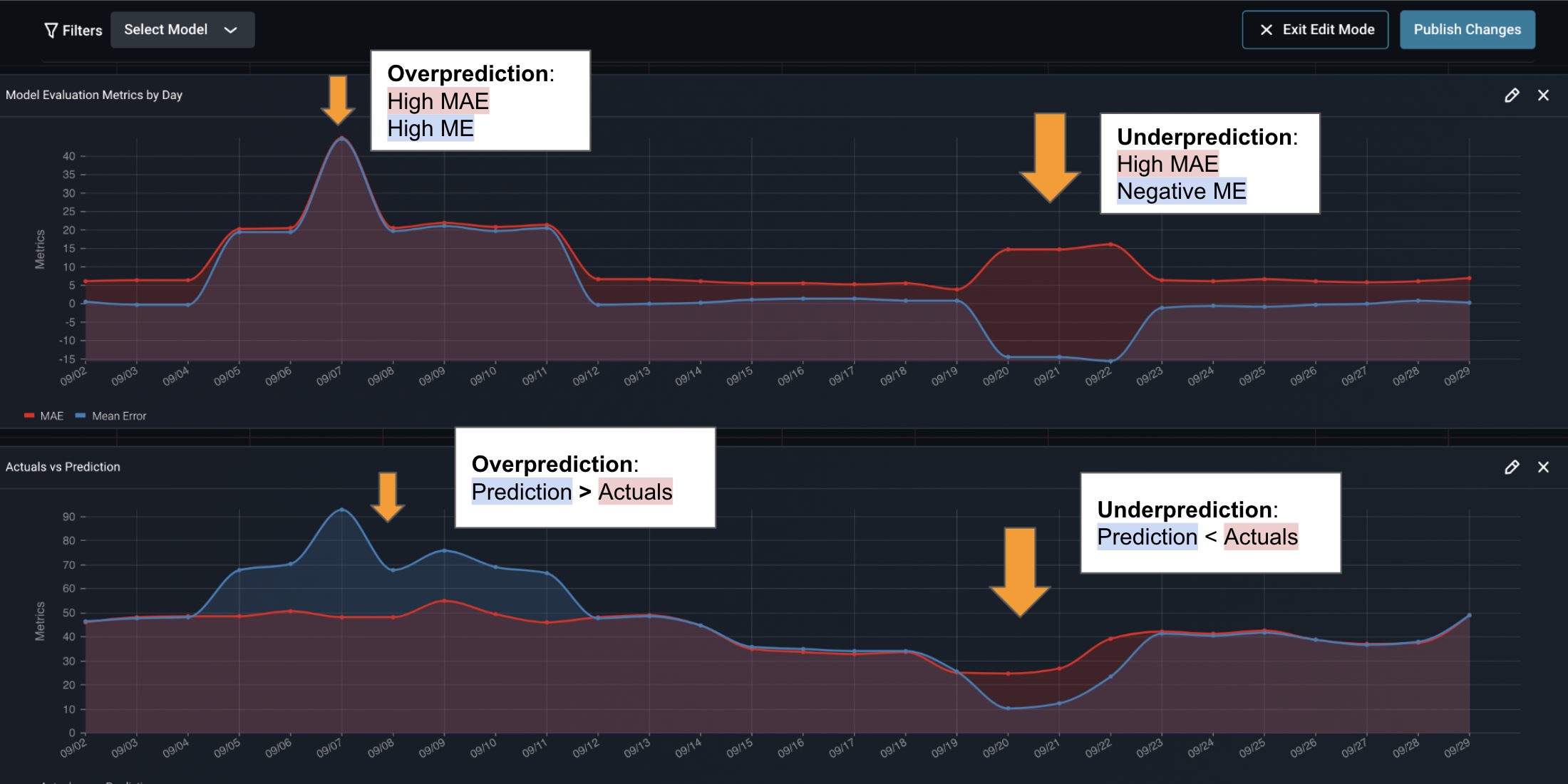
• Mean error (ME): average historical error (bias); a positive value signifies an overprediction, while a negative value means underprediction. While mean error isn’t typically the loss function that models optimize for in training, the fact that it measures bias is often valuable for monitoring business impact.
• Mean absolute error (MAE): the absolute value difference between a model’s predictions and ground truth, averaged out across the dataset. A great “first glance” at model performance since it isn’t skewed by extreme errors of a few predictions.
• Mean absolute percentage error (MAPE): measures the average magnitude of error produced by a model; one of the more common metrics of model prediction accuracy.
• Mean squared error (MSE): the difference between the model’s predictions and ground truth, squared and averaged out across the dataset. MSE is used to check how close the predicted values are to the actual values. As with root mean square error (RMSE), this measure gives higher weight to large errors and therefore may be useful in cases where a business might want to heavily penalize large errors or outliers.

It should be noted that mean error is not enough to tell the story of biases. In a feature drift event where there is both over-prediction and under-prediction in a given time period, mean error can be cancelled out by opposing metric values. That’s why it’s helpful to visualize the magnitude and direction of mean error and mean absolute error side-by-side — together, both can be used to identify when a model’s performance is subpar for a given time period.

All metrics have tradeoffs, and additional context can make a big difference in understanding whether a model is underperforming. In selecting which metrics are most useful to keep a close eye on, knowing the business outcome you are optimizing toward is paramount. A company hoping to avoid large underpredictions — like a retailer gearing up for a holiday period that constitutes most of its annual sales, for example — might optimize around root mean square error or mean square error and closely follow a graph with it and mean error to surface up issues of bias in predictions. In practice, observing all of the above metrics can have a tangible impact.

Identifying Performance Issues

Once it’s clear that a demand forecast is off-target based on bias and error metrics, teams can then identify the slices  — or combinations of features and values — driving a dip in performance. If a packaged food manufacturer has a high mean absolute error and a high mean error over a given time period, for example, it might be because a model’s training data contains more purchases from brand loyalists than are generally seen in the real world. From there, ML teams might upsample more sales data from people who prefer to buy generic products to retrain the model — or train a separate model for the lower-performing slice identified and segment the two models in production.

The Importance of Drift Detection, Diagnosis

As mentioned, monitoring and troubleshooting drift or distribution changes is critical, especially for regression demand forecasts given their complexity. Measuring population stability index as a distribution check, ML teams can detect changes in the distributions that might make a feature less valid as an input to the model.

If a major retailer has a high mean absolute error but a negative mean error, for example, it is likely  underpredicting demand. Diving deeper, the retailer’s ML team might discover this is caused by changing consumer preferences — say, shopping for holiday gifts earlier than in years past, and in larger sizes. Armed with this insight, they can retrain the model accordingly. By having an ML observability platform in place, organizations can quickly visualize and root cause these issues. That becomes all the more important during outlier events.

Conclusion

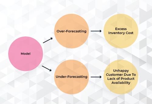
Given the changing nature of product development and global operations across industries in the wake of COVID-19, we may be witnessing a once-in-a-generation reset in the applications of demand forecasting models. Retailers, for instance, are likely more willing than in years past to be willing to take on extra inventory — viewing under-forecasting as more costly than over-forecasting due to the potential to lose out on customers.

ML observability can help teams optimize toward these outcomes, avoid costly mistakes and stay on top of fast-moving changes. By identifying the features contributing to over- or underpredictions and quickly getting to the bottom of issues, teams can ensure future forecasts are both accurate — and sunny.