


Using Statistical Distance Metrics for Machine Learning Observability

Aparna Dhinakaran
Co-founder & Chief Product Officer
Statistical Distances are used to quantify the distance between two distributions and are extremely useful in ML observability. This blog post will go into statistical distance measures and how they are used to detect common machine learning model failure modes.
Data problems in Machine Learning can come in a wide varietythat range from sudden data pipeline failures to long-term drift in feature inputs. Statistical distance measures give teams an indication of changes in the data affecting a model and insights for troubleshooting. In the real world post model-deployment, these data distribution changes can come in a myriad of different ways and cause model performance issues.
Here are some real-world data issues that we’ve seen in practice.
- Incorrect data indexing mistake — breaks upstream mapping of data
- Bad text handling — causes new tokens model has never seen
- Mistakes Handling Case
- Problems with New Text String
- Different sources of features with different coordinates or indexing
- 3rd Party data source makes a change dropping a feature, changing format, or moving data
- Newly deployed code changes an item in a feature vector
- Periodic daily collection of data fails, causing missing values or lack of file
- Software engineering changes the meaning of a field
- 3rd Party Library Functionality Changes
- Presumption of valid format that changes and is suddenly not valid
- Date string changes format
- System naturally evolves and feature shifts
- Outside world drastically changes (e.g., the COVID-19 pandemic) and every feature shifts
- Drastic increase in volume skews statistics
These are examples of data issues that can be caught using statistical distance checks.
Statistical distances can be used to analyze
- Model Inputs: Changes in inputs into a model, especially critical most important features or features that might be the output of an upstream model.
- Model Outputs: Changes in outputs of a model
- Actuals: Changes in actuals (ground truth received). In some cases, the ground truth might not be available within a short time horizon after prediction. In these cases, teams often use proxy metrics/data.
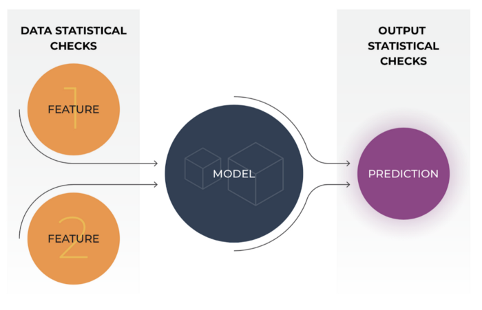
These checks are extremely insightful for model performance troubleshooting and they allow teams to get in front of major model issues before these problems affect business outcomes. In this image below, there are statistical checks that can be done on model inputs (features) and model outputs (predictions).
Statistical distance measures are defined between two distributions — distribution A and distribution B. One of these distributions is commonly referred to as the reference distribution (we will refer to this as distribution A) — this is what you are comparing against. The other distribution is typically the current state of the system that you are comparing to the reference distribution (we will refer to this as distribution B).
In the context of ML Observability, the reference distribution can be a number of different options. The first distinction to make is that the reference distribution can be a distribution across a fixed time window (distribution doesn’t change) or a moving time window (distribution can change).
In the image below, you can see that the examples of the fixed reference distribution include a snapshot of training distribution, initial model deployment distribution (or a time when the distribution was thought to be stable), and validation/test set distribution. An example of a statistical distance using a fixed reference distribution is to compare the model’s prediction distribution made from a training environment (distribution A) to the model’s prediction distribution from a production environment (distribution B).
The reference distribution can also be a moving window. In the image below, there are two examples where the reference distribution is a moving window — last week and A/B testing use cases. For the first example, one might want to compare the distribution of last week’s predictions to this week’s prediction. In this case, each week there will be a new reference distribution. If you are A/B testing two different model versions in production, you can compare if the prediction distribution from your champion model is similar to the prediction distribution from the challenger model.
The options for what you set as the reference distribution will depend on what you are trying to catch and we will dive into common statistical distance checks to set up for models.
Model Inputs
Model inputs can drift suddenly, gradually, or on a recurring basis depending on what is set as the reference distribution. As the old adage goes, “garbage in, garbage out.” In other words, a model is only as good as the data flowing into the model. If the input data changes and is drastically different than what the model has observed previously or has been trained on, it can be indicative that the model performance can have issues.
Here are a few statistical distance checks to set up on model inputs:
The distribution of a feature can drift over time in production. It is important to know if a feature distribution has changed over time in production and if this is impacting the model. In this setup, the reference distribution (distribution A) is the feature distribution in training. The current window (distribution B) can be set to the feature distribution over a certain time window (ex: a day, a week, a month, etc). If the feature distribution is highly variant, it can be helpful to set a longer lookback window so the statistical distance check can be less noisy.
2. Feature Distribution in Production Time Window A vs Feature Distribution in Production Time Window B
It can also be useful to set up distribution checks on a feature at two different intervals in production. This distribution check can focus on more short-term distribution changes compared to the training vs production check. If setting the training distribution as the reference distribution, setting a short production time window can be noisy if there are any fluctuations (ex: traffic patterns, seasonal changes, etc). Setting up a statistical distance check against last week vs the current week can give an indication of any sudden outliers or anomalies in the feature values. These can also be extremely useful to identify any data quality issues that might get masked by a larger time window.
Identifying if there has been a distribution change in the feature can give early indications of model performance regressions or if that feature can be dropped if it’s not impacting the model performance. It can lead to model retraining if there are significant impacts to the model performance. While a feature distribution change should be investigated, it does not always mean that there will be a correlated performance issue. If the feature was less important to the model and didn’t have much impact on the model predictions, then the feature distribution change might be more of an indication it can be dropped.
Teams in the real world use model input checks to determine when models are growing stale, when to retrain models, and slices of features that might indicate performance issues. One team I spoke to that uses a financial model for underwriting generates analysis on feature stability by comparing the feature in production to training to make sure the model decisions are still valid.
Model Outputs
Just like model inputs can drift over time, model outputs distributions can also change over time. Setting statistical distance checks on model predictions make certain the outputs of the model are not drastically different than their reference distributions.
3. Prediction Distribution in Training vs Prediction Distribution in Production
The goal of output drift is to detect large changes in the way the model is working relative to training. While these are extremely important to ensure that models are acting within the boundaries previously tested and approved, this does not guarantee that there is a performance issue. Similar to how a feature distribution change does not necessarily mean there is a performance issue, prediction distribution changes doesn’t guarantee there is a performance issue. A common example is if a model is deployed to a new market, there can be distribution changes in some model inputs and also the model output.
4. Prediction Distribution at Production Time Window A vs Prediction Distribution in Production Time Window B
Similar to model inputs, the prediction distribution can also be monitored to another time window in production. One team we talked with, who was evaluating a spam filter model, uses the distribution of the output of the model versus a fixed time frame to surface changes in attack patterns that might be getting through the model. The reference distribution here can either be a moving time window or a fixed time frame. A common fixed time frame we hear is using the initial model launch window.
5. Prediction Distribution for Model Version A vs Prediction Distribution for Model Version B at Same Time Window
Teams that have support for canary model deployment can set up statistical distance checks on the prediction distributions for different model versions. While A/B testing two different models in production with each model receiving a certain amount of traffic or backtesting a model on historical data, comparing the prediction distribution gives insight into how one model performs over another.
Model Actuals
6. Actuals Distribution at Training vs Actuals Distribution in Production
Actuals data might not always be within a short-term horizon after the model inferences have been made. However, statistical distance checks on actual distributions help identify if the structure learned from the training data is no longer valid. A prime example of this is the Covid-19 pandemic causing everything from traffic, shopping, demand, etc patterns to be vastly different today from what the models in production had learned before the pandemic began. Apart from just large-scale shifts, knowing if the actuals distribution between training data vs production for certain cohorts can identify if there
Model Predictions vs Actuals
7. Predictions Distribution at Production vs Actuals Distribution at Production
This statistical distance check is comparing production distribution of predictions vs actuals. This can help catch performance issues by pinpointing specific cohorts of predictions that have the biggest difference from their actuals. These checks can sometimes catch issues that are masked in averages such as MAE or MAPE.
We just covered common use cases for statistical distances. There are a number of different statistical distance measures that quantify change between distributions. Different types of distance checks are valuable for catching different types of issues. In this blog post, we will cover the following 4 distance measures and when each can be most insightful.
PSI
The PSI metric has many real-world applications in the finance industry. It is a great metric for both numeric and categorical features where the distributions are fairly stable.
Equation:PSI = (Pa — Pb)ln(Pa/Pb)PSI is an ideal distribution check to detect changes in the distributions that might make a feature less valid as an input to the model. It is used often in finance to monitor input variables into models. It has some well-known thresholds and useful properties.