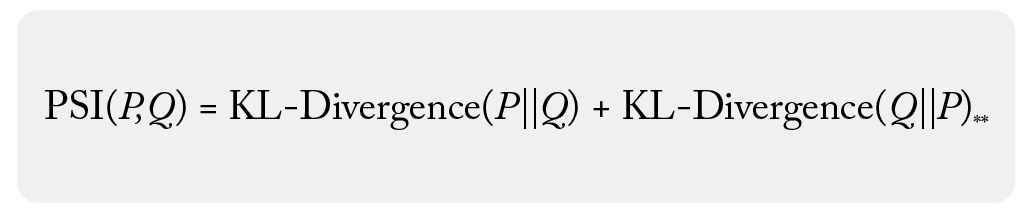
Population Stability Index (PSI): What You Need To Know

Population stability index (PSI) is a statistical measure with a basis in information theory that quantifies the difference between one probability distribution from a reference probability distribution. The advantage of PSI over KL divergence is that it is a symmetric metric. PSI can be thought of as the round trip loss of entropy – the KL Divergence going from one distribution to another, plus the reverse of that.

What Is Population Stability Index (PSI)?

Population stability index is a symmetric metric that measures the relative entropy, or difference in information represented by two distributions. It can be thought of as measuring the distance between two data distributions showing how different the two distributions are from each other.

The following shows the symmetry with KL Divergence:

There is both a continuous form of PSI

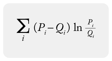
And a discrete form of PSI

For additional reference, Bilal Yurdikal authored one of the better technical papers on PSI.

In model monitoring, we almost exclusively use the discrete form of PSI and obtain the discrete distributions by binning data. The discrete form of PSI and continuous forms converge as the number of samples and bins limit move to infinity. There are optimal selection approaches to the number of bins to approach the continuous form.

✏️NOTE: In practice, the number of bins can be far less than the above number implies – and how you create those bins to handle the case of 0 sample bins is more important practically speaking than anything else (stay tuned for future content addressing how to handle zero bins naturally).

How Is PSI Used In Model Monitoring and Observability?

In model monitoring, PSI is used to monitor production environments, specifically around feature and prediction data. PSI is also utilized to ensure that input or output data in production doesn’t drastically change from a baseline. The baseline can be a production window of data or a training/validation dataset.

Drift monitoring can be especially useful for teams that receive delayed ground truth to compare against production model decisions. Teams rely on changes in prediction and feature distributions as a proxy for performance changes. PSI was picked up by the finance industry as a key metric used to measure feature drift and is one of the more stable and useful drift metrics.

PSI is typically applied to each feature independently; it is not designed as a covariant feature measure but rather a metric that shows how each feature has diverged independently from the baseline values.

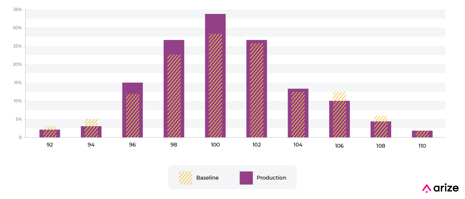
The p(x) shown above in orange stripes is the reference or baseline distribution. The most common baselines are either a trailing window of production data or the training datasets. Each bin additively contributes to PSI. The bins jointly add up to the total percent distribution.

✏️NOTE: sometimes non-practitioners have a somewhat overzealous goal of perfecting the mathematics of catching data changes. In practice, it’s important to keep in mind that real data changes all the time in production and many models extend well to this modified data. The goal of using drift metrics is to have a solid, stable, and strongly useful metric that enables troubleshooting.

Is PSI A Symmetric Metric?

PSI is a symmetric metric. If you swap the baseline distribution p(x) and sample distribution q(x), you will get the same number. This has a number of advantages compared to KL divergence for troubleshooting data model comparisons. There are times where teams want to swap out a comparison baseline for a different distribution in a troubleshooting workflow, and having a metric where A / B is the same as B / A can make comparing results much easier.

This is one reason Arize’s model monitoring platform defaults to population stability index (PSI) – a symmetric derivation of KL Divergence – as one of the main metrics to use for model monitoring of distributions.

Differences Between Continuous Numeric and Categorical Features

PSI can be used to measure differences between numeric distributions and categorical distributions.

Numerics

In the case of numeric distributions, the data is split into bins based on cutoff points, bin sizes and bin widths. The binning strategies can be even bins, quintiles, and complex mixes of strategies that ultimately affect PSI (stay tuned for a future write-up on binning strategy).

Categorical

The monitoring of PSI tracks large distributional shifts in the categorical datasets. In the case of categorical features, often there is a size where the cardinality gets too large for the measure to have much usefulness. The ideal size is around 50-100 unique values – as a distribution has higher cardinality, the question of how different the two distributions are and if it really matters gets muddied.

High Cardinality

In the case of high cardinality feature monitoring, out-of-the-box statistical distances do not generally work well. Instead, Arize typically recommends two options:

1. Embeddings: In some high cardinality situations, the values being used – such as User ID or Content ID – are already used to create embeddings internally. Arize embedding monitoring can help.
2. Pure High Cardinality Categorical: In other cases, where the model has encoded the inputs to a large space, just monitoring the top 50-100 top items with PSI and all other values as “other” can be useful.

Sometimes what you want to monitor is something very specific, such as the percent of new values or bins in a period. These can be setup more specifically with data quality monitors.

PSI Example

Here is an example of PSI with numeric and categorical features.

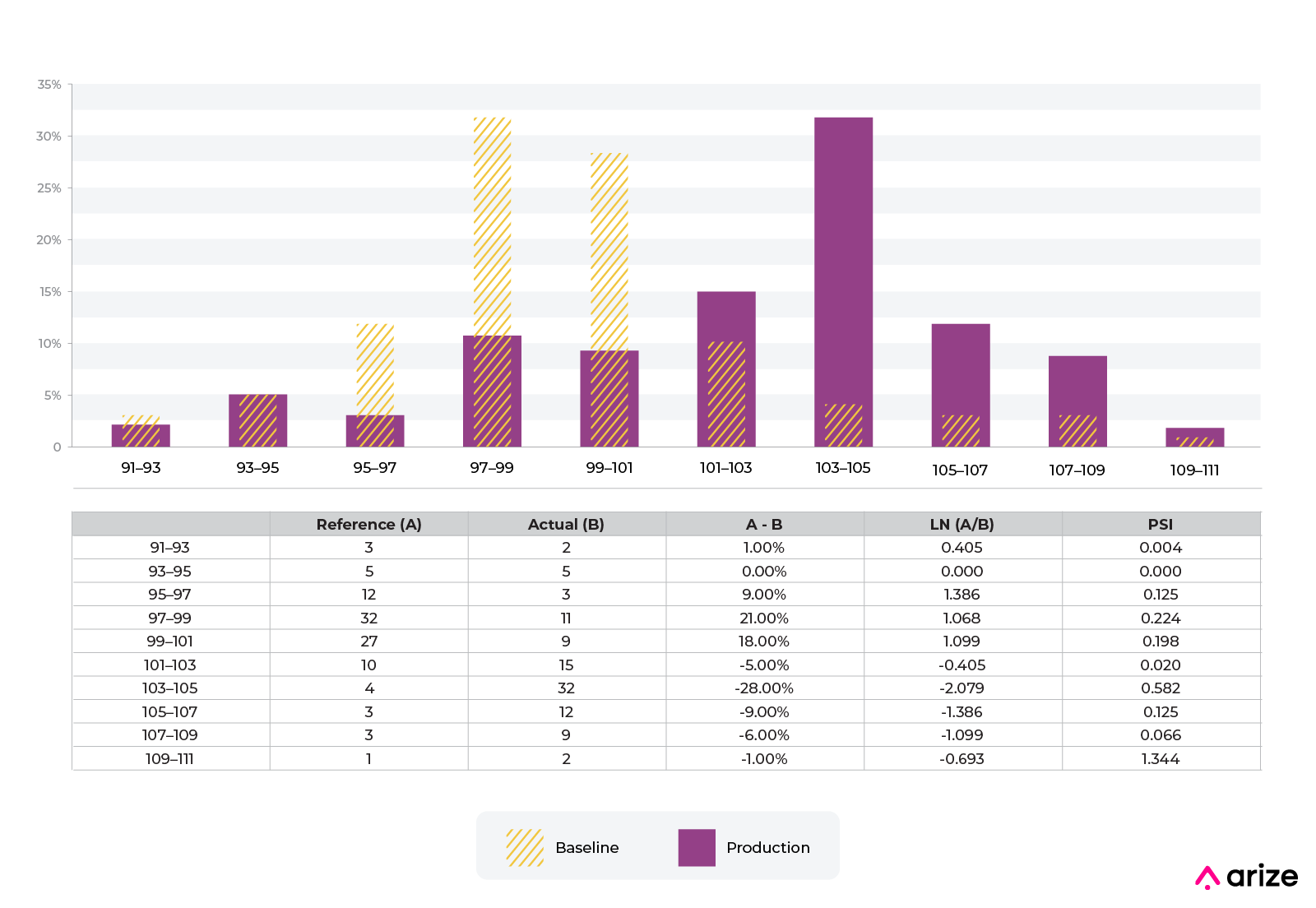
Imagine we have a numeric distribution of charge amounts for a fraud model. The model was built with the baseline shown in the picture above from training. We can see that the distribution of charges has shifted. There are a number of industry standards around thresholds, but often using a production trailing value to set an auto threshold is the best option. There are many examples in production where the fixed setting of 0.2 doesn’t make sense.

The example shows a categorical variable and PSI over the distribution. Note the movement in one category or bin of 5%, for example, causes a corresponding bin set that decreases by 5%. This is going to be true of every distribution and every grouping of bins that are normalized.

Intuition Behind PSI

It’s important to have a bit of intuition around the metric and changes in the metric based on distribution changes.

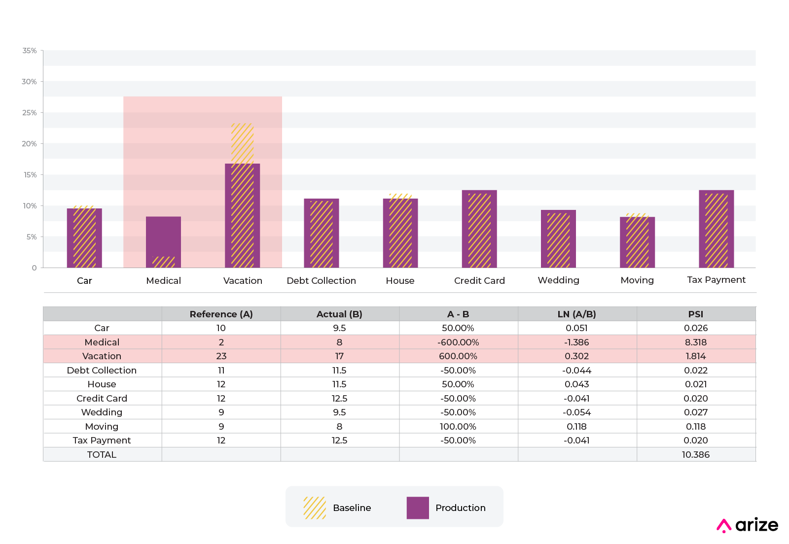
The above example shows a move from one categorical bin to another. The predictions with “medical” as input on a feature (use of loan proceeds) increased from 2% to 8%, while the predictions with “vacation” decreased from 23% to 17%.

In this example, the component to PSI related to “medical” is 8.318 and is larger than the component for the “vacation” percentage movement of 1.814.

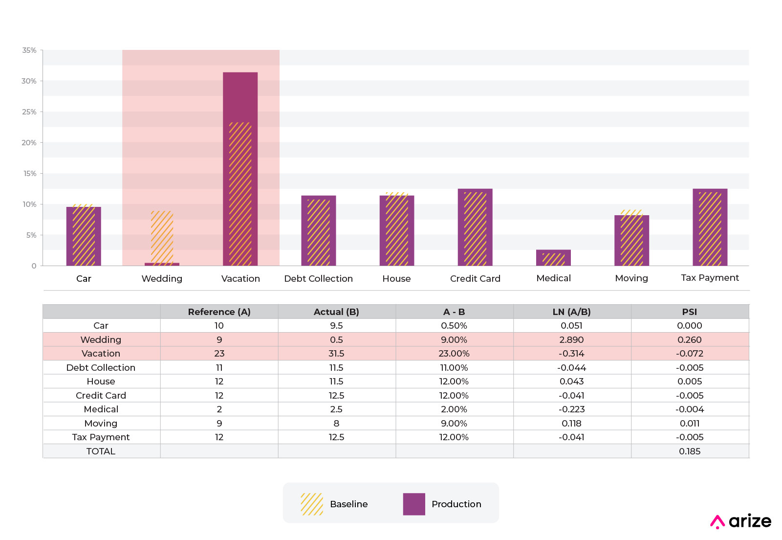
Here is a spreadsheet for those that want to play with and modify these percentages to better understand the intuition.

Conclusion

PSI is a common way to measure drift. Hopefully this guide on best practices for using PSI in monitoring data movements is helpful. Additional pieces will cover binning challenges and other recommended drift metrics.