


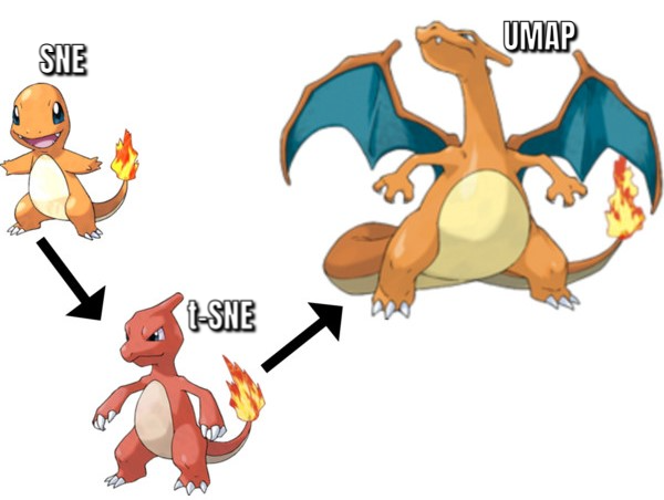
There are several prominent ways to visualize the embedding representation of a dataset using dimensional reduction techniques. This post summarizes three popular dimensionality reduction techniques and their evolution.
It is worth noting at the outset that the academic papers introducing these techniques — SNE (“Stochastic Neighbor Embedding” by Geoffrey Hinton and Sam Roeweis), t-SNE (“Visualizing Data using t-SNE” by Laurens van der Maaten and Geoffrey Hinton), and UMAP (“Umap: Uniform manifold approximation and projection for dimension reduction” by Leland McInnes, John Healey, and James Melville) — are worth reading in full. That said, these are dense papers. This lesson is intended to be a digestible guide – maybe a first step before reading the complete papers – for time-strapped ML practitioners to help them understand the underlying logic and evolution from SNE to t-SNE to UMAP.
What Is Dimensionality Reduction?
Dimension reduction plays an important role in data science as a fundamental technique in both visualization and pre-processing for machine learning. Dimension reduction methods map high dimensional data X={x0, x1, …, xN} into lower dimensional data Y = {y0, y1, …, yN} with N being the number of data points.
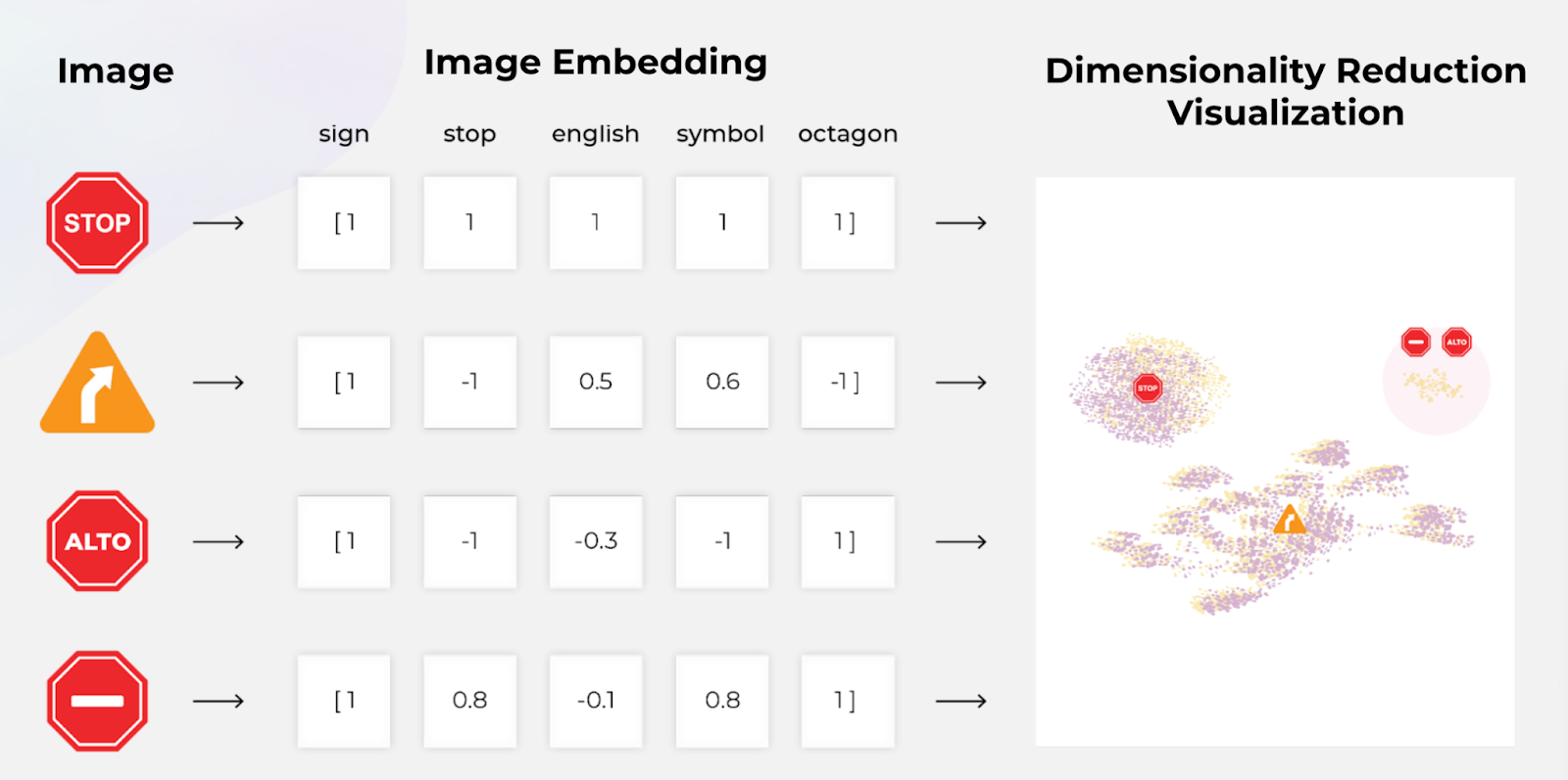
In essence, computing embeddings is a form of dimension reduction. When working with unstructured data, the input space can contain images of size WHC (Width, Height, Channels), tokenized language, audio signals, etc. For instance, let the input space be composed of images with resolution 1024×1024. In this case, the input dimensionality is larger than one million. Let’s assume you use a model such as ReNet or EfficientNet and extract embeddings with 1000 dimensions. In this case your output space dimensionality is 1000, three orders of magnitude lower! This transformation turns the very large, often sparse, input vectors into smaller (still of considerable size), dense feature vectors, or embeddings. Hence, we will refer to this subspace as the feature space or embedding space.
Once we have feature vectors associated with our inputs, what do we do with them? How can we obtain human interpretable information from them? We can’t visualize objects in higher than three dimensions. Hence, we need tools to further reduce the dimensionality of the embedding space down to two or three, ideally preserving as much of the relevant structural information of our dataset as possible.
There are an extensive amount of dimensionality reduction techniques. They can be grouped into three categories: feature selection, matrix factorization, and neighbor graphs. We will focus on the latter category, which includes SNE (Stochastic Neighbor Embedding), t-SNE (t-distributed Stochastic Neighbor Embedding) and UMAP (Uniform Manifold Approximation and Projection).
SNE vs t-SNE vs UMAP
In this section, we will follow the evolution of neighbor graphs approaches starting with SNE. Then, we will build from it and explain the modifications applied that resulted in t-SNE and later on in UMAP.
The three algorithms operate roughly in the same way:
- Compute high dimensional probabilities p.
- Compute low dimensional probabilities q.
- Calculate the difference between the probabilities by a given cost function C(p,q).
- Minimize the cost function.
SNE
This section covers the Stochastic Neighbor Embedding (SNE) algorithm. This will be the building block from which we’ll develop a better understanding of t-SNE and UMAP.
Step 1: Calculate the High Dimensional Probabilities
We start by computing the probability pj|i that the data point i would pick another point j as its neighbor,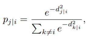
where dj|i2 represents the dissimilarity between high dimensional points xi, xj. It is defined as the scaled Euclidean distance,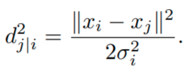
Mathematical intuition: Given two points xi, xj, the farther they are, the higher their distance dj|i, the higher their dissimilarity, and the lower the probability that they will consider each other neighbors. Key concept: the further away two embeddings are in the space, the more dissimilar they are.
Note that the dissimilarities are not symmetric due to the parameter σi. In practice, the user sets the effective number of local neighbors or perplexity. Once the perplexity, k, is chosen, the algorithm finds σi by a binary search to make the entropy of the distribution over neighbors equal log2k: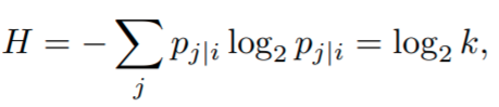
where H is the Shannon entropy, measured in bits. From the previous equation we can obtain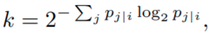
so that by tuning σi, we tune the right hand side until it matches the perplexity set by the user. The higher the effective number of local neighbors (perplexity), the higher σi and the wider the Gaussian function used in the dissimilarities.
Mathematical intuition: The higher the perplexity, the more likely it is to consider points that are far away as neighbors.
One question may arise: if the perplexity is user-determined, how do we know which one is correct? This is where art meets science. The choice of perplexity is crucial for a useful projection into a low-dimensional space that we can visualize using a scatter plot. If we pick too low of a perplexity, clusters of data points that we expect to be together given their similarity will not appear together and we will see subclusters instead. On the other hand, if we pick a perplexity too large for our dataset, we will not see correct clustering, since points from other clusters will be considered neighbors. There isn’t a definite all-good value for the perplexity. However, there are good rules of thumb.
Advice: The creators of SNE and t-SNE (yes, t-SNE has perplexity as well) use perplexity values between five and 50.
Since in many cases, there is no way to know what the correct perplexity is, getting the most from SNE (and t-SNE) may mean analyzing multiple plots with different perplexities.
Step 2: Calculate the Low Dimensional Probabilities
Now that we have the high dimensional probabilities, we move on to calculate the low dimensional ones, which depend on where the data points are mapped in the low dimensional space. Fortunately, these are easier to compute since SNE also uses Gaussian neighborhoods but with fixed variance (no perplexity parameter),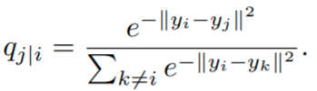
Step 3: Choice of Cost Function
If the points yi are placed correctly in the low-dimensional space, the conditional probabilities p and q will be very similar. To measure the mismatch between both probabilities, SNE uses the Kullback-Leibler divergence as a loss function for each point. Each point in both high and low dimensional space has a conditional probability to call another point its neighbor. Hence, we have as many loss functions as we have data points. We define the cost function as the sum of the KL divergences over all data points,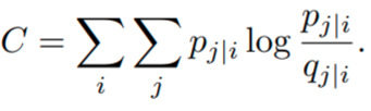
The algorithm starts by placing all the yi in random locations very close to the origin, and then is trained minimizing the cost function C using gradient descent. Details about the differentiation of the cost function is beyond the scope of this post.
It’s worth developing some intuition about the loss function used. The algorithm’s authors state that “while SNE emphasizes local distances, its cost function cleanly enforces both keeping the images of nearby objects nearby and keeping the images of widely separated objects relatively far apart.” Let’s see if this is true using the next figure where we see the KL divergence for the high and low dimensional probabilities p and q, respectively.
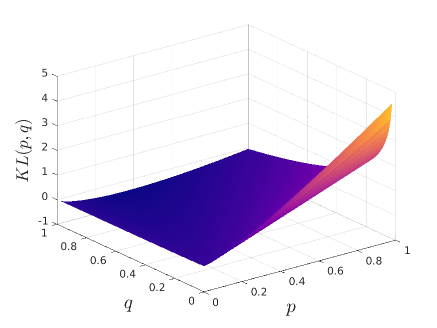
If two points are close together in high dimensional space, their dissimilarities are low and the probability p should be high (p ~ 1). Then, if they were mapped far away, the low dimensional probability would be low (q ~ 0). In this scenario we can see that the loss function takes very high values, severely penalizing that mistake. On the other hand, if two points are far from each other in high dimensional space, their dissimilarities are high and the probability p should be low (p ~ 0). Then, if they were mapped near each other, the low dimensional probability would be high (q ~ 1). We can see that the KL divergence is not penalizing this mistake as much as we would want. This is a key issue that will be solved by UMAP.
t-SNE
At this point we have a good idea of how SNE works. However, the algorithm has two problems that t-SNE tries to solve: its cost function is very difficult to optimize, and it has a crowding problem (more on this below). Two main modifications are introduced by t-SNE to solve these issues: symmetrization and the use of t-distributions for the low-dimensional probabilities, respectively. These modifications arguably made t-SNE the state-of-the-art for dimension reduction for visualization for many years until UMAP came along.
Symmetric SNE
The first modification is the use of a symmetrized version of SNE. Generally, the conditional probabilities described so far are not symmetric. This means that the probability of point xi to consider point xj as its neighbor is not the same probability that point xj would consider point xias a neighbor. We symmetrize pairwise probabilities in high dimensional space by defining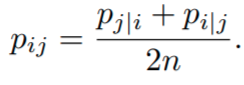
This definition of pij is such that every data point xi makes a non negligible contribution to the cost function. You might be wondering, what about the low dimensional probabilities?
The Crowding Problem
With what we have so far, if we want to correctly project close distances between points, the moderate distances are distorted and appear as huge distances in the low dimensional space. This is because “the area of the two-dimensional map that is available to accommodate moderately distant data points will not be nearly large enough compared with the area available to accommodate nearby data points.”
To solve this, the second main modification introduced is the use of the Student t-Distribution (which is what gives the ‘t’ to t-SNE) with one degree of freedom for the low-dimensional probabilities,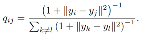
Now the pairwise probabilities are symmetric (pij = pji and qij = qji). The main advantage is that the gradient of the symmetric cost function,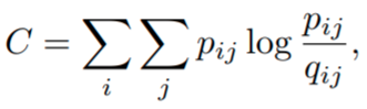
has a simpler form and is much easier and faster to compute, improving performance.
Since t-SNE also uses KL divergence as its loss function, it also carries the problems discussed in the previous section. This is not to say that it is completely ignored, but the main takeaway is that t-SNE severely prioritizes the conservation of the local structure.
Intuition: Since the KL divergence function does not penalize the misplacement in low dimensional space of points that are far away in high dimensional space, we can conclude that the global structure is not well preserved. t-SNE will group similar data points together into clusters, but distances between clusters might not mean anything.
UMAP
Uniform Manifold Approximation and Projection (UMAP) for dimension reduction has many similarities with t-SNE as well as some very critical differences that have made UMAP our preferred choice for dimension reduction.
The paper introducing the technique is not for the faint of heart. It details the theoretical foundations for UMAP, based in manifold theory and topological data analysis. We will not go into the details of the theory but keep this in mind: the algorithmic decisions in UMAP are justified by strong mathematical theory, which ultimately will make it such a high quality general purpose dimension reduction technique for machine learning.
Now that we have an understanding of how t-SNE works, we can build on that and talk about the differences with UMAP and the consequences of those differences.
A Graph of Similarities
Unlike t-SNE that works with probabilities, UMAP works directly with similarities.
High dimensional similarities:
Low dimensional similarities: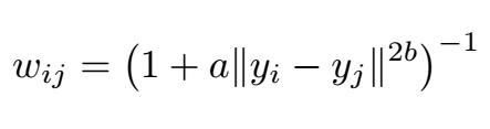
Note that in both cases there is no normalization (no denominator) applied, unlike t-SNE, with the corresponding improvement in performance. The symmetrization of the high dimensional similarities is carried out using probabilistic t-conorm:
In addition, UMAP allows for different choice of metric functions d for the high dimensional similarities (eq). We need to address the meaning of ρi and σi. The former represents the minimum desired separation between close points in the low dimensional space, and the latter is set to be the value such that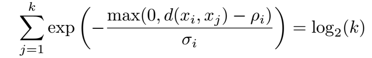
where k is the number of nearest neighbors. Both the ρi and σi are hyper-parameters with effects that will be discussed at the end of the section.
Optimization Improvements
In the optimization phase of the algorithm, the creators of UMAP made some design decisions that played a crucial role in its great performance, including:
- UMAP uses cross entropy as loss function, while t-SNE uses KL divergence. The CE loss function has both attractive and repulsive forces, while KL only has attractive (It is worth noting that t-SNE has repulsive forces but not on the loss function. The repulsive forces appear in the renormalization process of the similarity matrix. However, global renormalization is very expensive, UMAP has it simpler by using CE loss and with better results on preserving global structure). With this new choice of loss function, placing objects that are far away in high-dimensional space nearby in the low-dimensional space is penalized. Thanks to the better choice of loss function, UMAP can capture more of the global structure than its predecessors.
- UMAP uses stochastic gradient descent to minimize the cost function, instead of the slower gradient descent.

(a)- KL loss used by t-SNE
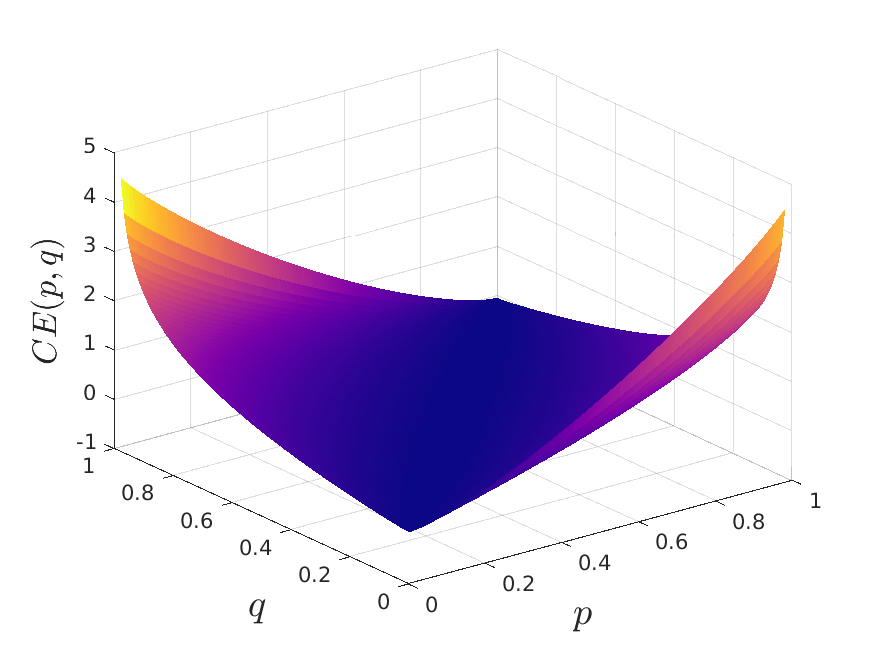
(b)– CE loss used m
Choice of Initialization
UMAP uses spectral initialization, not random initialization of the low dimensional points. A very convenient Laplacian Eigenmaps initialization (followed from the theoretical foundations). This initialization is relatively quick, since it is obtained from linear algebra operations. It provides a good starting point for stochastic gradient descent. This initialization is, in theory, deterministic. However, given the large sparse matrices involved, computational techniques provide approximate results. As a consequence, determinism is not guaranteed but great stability is achieved. This initialization provides faster convergence as well as greater consistency, i.e., different runs of UMAP will yield similar results.
There are other differences that are worth exploring. Moreover, UMAP comes with several disadvantages. Stay tuned for an upcoming piece on the pros and cons of UMAP.
Conclusion
Techniques for visualizing embeddings have come a long way in the past few decades, with new algorithms made possible by the successful combination of mathematics, computer science and machine learning. The evolution from SNE to t-SNE and UMAP opens up new possibilities for data scientists and machine learning engineers to better understand their data and troubleshoot models.
Get Started
Want to learn more? Read about monitoring unstructured data. Want to try out embedding analysis and embedding drift monitoring leveraging UMAP 2D and 3D visualizations? Sign up for a free Arize account.