

TL;DR
- LLM evaluation cost extends beyond judge tokens. Trace volume, evaluator coverage, workflow depth, human review, and retention all contribute to the total bill.
- Offline evals are easier to forecast because teams control the dataset and experiment scope. Production evals inherit live traffic, variable trace depth, and changing failure patterns.
- Production cost is best controlled through sampling, filtering, selective scoring surfaces, and evaluator routing. Expensive judges and human review should be reserved for uncertain or consequential cases.
- Evaluation spend earns its return when it prevents repeated failures, shortens debugging, and gives teams stronger evidence for deciding what to ship.
LLM evaluation is easy to budget in development. Teams control the dataset, evaluators, models, and number of experiment runs.
Production evaluation has a different cost model. Live traffic changes, traces vary in depth, agent workflows create more scoring surfaces, and some failures still need human review.
Judge tokens are the easiest cost to count. They are only one part of the bill. Trace processing, evaluator runs, retention, annotation, and repeated experiments can all increase the total cost of evaluation.
A strong LLM evaluation system uses the cheapest reliable signal for each task. Code-based checks can validate structure and tool arguments. LLM-as-a-judge can score open-ended qualities such as relevance or groundedness. Human review can handle calibration and high-risk failures.
This guide breaks down where evaluation costs come from, why production changes the economics, and how teams can control spend without weakening release quality.
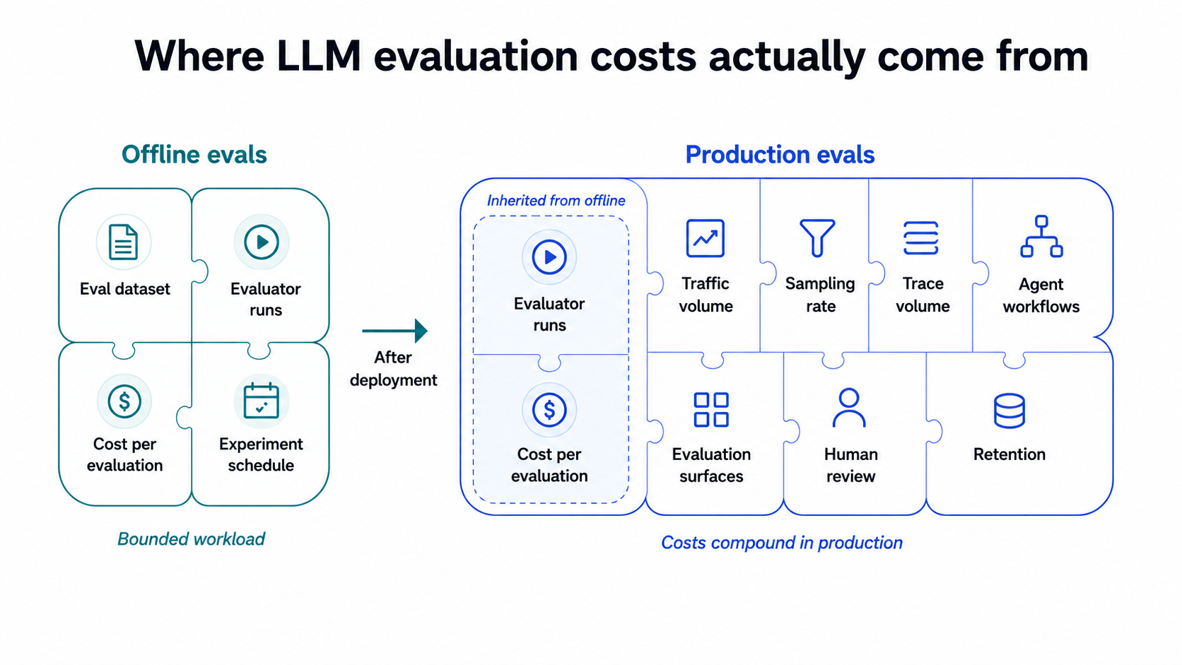
Evaluation cost follows the lifecycle of the application. Before deployment, teams choose the workload they want to evaluate. After deployment, live traffic and workflow behavior begin setting that workload for them.
Where LLM evaluation costs actually come from
LLM evaluation cost rarely appears as one clean line item. A team may see judge-token spend first, but the full cost builds across evaluator runs, trace volume, workflow depth, review overhead, and the systems needed to preserve evaluation history.
The cost model also changes across the application lifecycle. Offline evals run against a bounded workload that teams define in advance. Production evals inherit part of that same structure, then add live traffic, more evaluation surfaces, human review, and retention requirements.
Build better agents with Arize
Trace, evaluate, and learn. Build agents that work with Arize AX and start tracing your runs today.
Prefer open source? Try Arize Phoenix for self-hosted, open source agent observability.

Offline evals have a fixed cost model
Offline LLM evaluation starts with a workload the team can define in advance. During pre-production LLM evaluation, teams choose the eval dataset, candidate models, evaluators, repetitions, and experiment schedule before a run begins.
A simple cost model looks like:
Offline eval cost = dataset size × system variants × evaluator runs × cost per evaluation
Every variable can be controlled. A team can run a broad regression suite before a major release, use a smaller dataset during prompt iteration, or reserve expensive LLM judges for cases that require semantic judgment.
The main cost decision is how much evaluation each development stage actually needs. Running every evaluator across every example and every experiment can create a large bill without producing equally useful information.
Teams can control offline eval costs by matching evaluation depth to the decision being made. Early prompt experiments may need a small representative dataset. Release candidates may justify broader regression testing. High-risk workflows may need stronger judges, repeated runs, or human review.
Production evals have a moving cost model
Production evaluation starts with a less predictable workload. Traffic changes over time, traces do not all contain the same number of steps, and different failures may require different evaluation methods.
A simple production cost model looks like:
Production eval cost = traffic volume × sampling rate × evaluation surfaces × evaluator cost + human review + retention
Each part of that model can move independently.
| Cost driver | What changes in production | Cost implication |
|---|---|---|
| Traffic volume | Request volume rises, falls, or spikes | More traces become eligible for evaluation |
| Sampling rate | Teams evaluate all traffic or a selected percentage | Higher coverage creates more evaluator runs |
| Evaluation surfaces | A request may contain retrieval, routing, tool calls, and a final response | One user request can generate several evaluation targets |
| Evaluator choice | Checks may use code, smaller models, stronger judges, or humans | Cost per evaluation varies by method |
| Human review | Some failures need calibration, escalation, or domain expertise | Review cost depends on queue volume and reviewer type |
| Retention | Teams keep traces, scores, annotations, and release history | Storage and data access become part of total cost |
Production traffic therefore creates two planning problems. Teams need to decide how much traffic to evaluate and how deeply to evaluate each trace.
A simple chatbot may only need a sampled final-response evaluator. An agent workflow may need separate checks for retrieval, routing, tool selection, parameter extraction, recovery behavior, and final task success.
Production evaluation cost therefore follows the shape of the application and the traffic passing through it. The next cost is easier to see because it arrives directly on the model bill: judge tokens.
Judge tokens are the easiest cost to count
LLM judges create a relatively visible cost because every evaluation run is another inference workload. Each evaluated item fills the judge prompt with application data, the judge model processes that prompt, and the result returns as a label, score, and optional explanation.
In Arize AX, an LLM judge is configured around a few concrete pieces:
- Input fields: application inputs, outputs, metadata, or prompt variables selected from the span or trace being evaluated.
- Prompt template: the evaluation criteria and the variables passed to the judge.
- Judge configuration: the model, provider, and model parameters used for the evaluation.
- Output fields: the label, numerical score, and optional explanation returned by the judge.
The average cost of one judge run depends on the prompt tokens, completion tokens, model, and provider. AX tracks token usage and cost using fields such as:
llm.token_count.promptllm.token_count.completionllm.cost.completionllm.cost.total
Those fields allow cost to be inspected at the individual LLM-call level and aggregated across a complete trace.
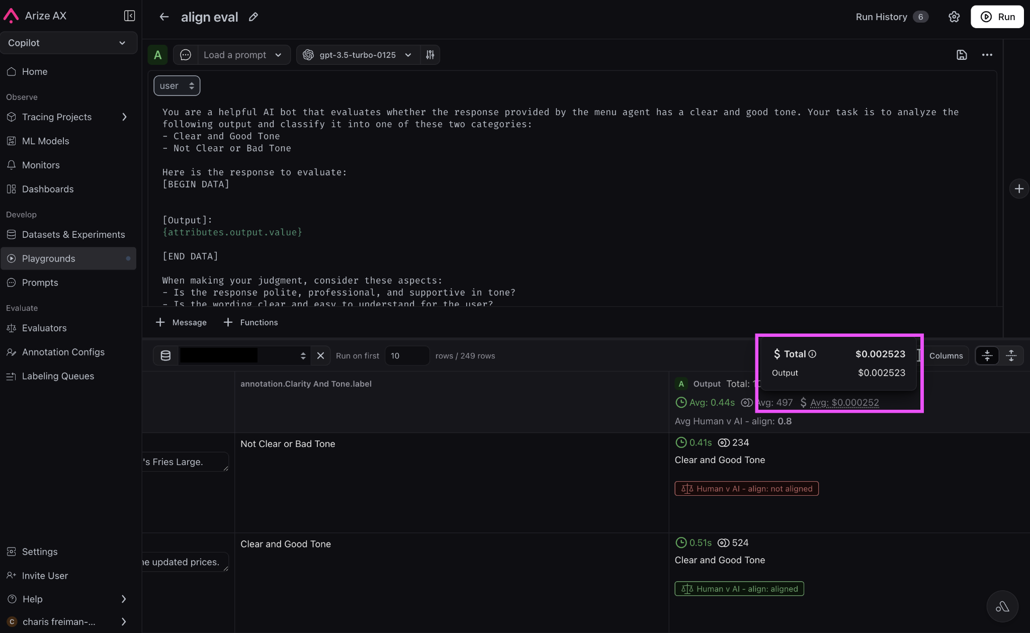
The Playground view makes judge spend directly inspectable during experiments. Production tasks use the same underlying token and pricing information, while sampling rate and evaluator coverage determine how often those judge calls run.
Consider a production dataset with 100,000 eligible responses. Evaluating 10% of them with one correctness judge creates 10,000 judge runs. Running correctness, groundedness, and policy evaluators on the same sample creates 30,000. Evaluating additional spans inside each trace increases the count again.
The price of one judge call may be easy to calculate. The harder question is how many judges the evaluation design creates.
Trace volume becomes the real multiplier
Trace volume multiplies production evaluation cost because every eligible trace can trigger one or more evaluator runs. Sampling rate controls how many traces are scored. Filtering controls which production traffic receives that coverage.
In AX, online evaluation tasks can run at span, trace, or session granularity. Teams can set a sampling rate and filter traffic by span kind, model name, metadata, or span attributes. Those controls let broad monitoring run at a lower rate while narrower tasks concentrate evaluation on specific workflows or failure classes.
Production traffic also changes composition over time. Parker Seegmiller and Sarah Masud Preum studied this problem in Measuring Distribution Shift in User Prompts and Its Effects on LLM Performance. The LENS study covered 192 post-deployment prompt-shift settings across time, user groups, and geography, using 4.68 million training prompts and 57,600 evaluation prompts.
The results were stark. Models fine-tuned on the original traffic lost an average of 73% of head-to-head comparisons against oracle models trained on the shifted prompt distributions.
The damage also varied sharply by axis. Temporal shift was the mildest, with loss rates around 44%. Shifts across user groups and geography were far more destructive, pushing loss rates to 87% and 88%.
The chart below shows the temporal axis. Both prompt shift and model degradation climb steadily as evaluation moves further from the training window, and this is the gentlest of the drift patterns the paper measured.
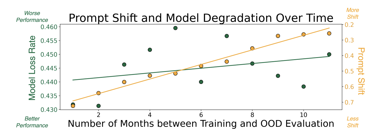
The finding changes how teams should think about trace coverage. A stable random sample can control judge spend while the underlying traffic mix continues to evolve. A support application, for example, may spend most evaluator calls on routine account-recovery conversations while a lower-volume billing workflow or regional user group develops a new failure pattern.
Sampling answers how much production traffic to evaluate. Task scope and filters answer which traffic deserves that spend. Efficient production evaluation combines broad baseline coverage with denser evaluation for risky, changing, or diagnostically valuable slices.
Agent workflows create more scoring surfaces
Agent workflows change evaluation economics because one user request can contain several decisions before the final response. A single task may pass through routing, retrieval, tool selection, parameter extraction, execution, retries, and reflection.
Each stage creates a different failure surface. Agent evaluation can separate router accuracy, tool selection, parameter extraction, skill quality, and path behavior instead of reducing the workflow to one final-response score.
Deeper workflows therefore create more places where evaluators could run. A chatbot may need one final-response check, while an agent may need targeted checks at several points in the same trace.
Teams control that cost by choosing the surfaces tied to expensive or consequential failures. Routine intermediate steps can remain observable without becoming separate judge calls.
Route evaluation depth where it earns its cost
Routing is most useful when evaluation tasks stop as soon as enough evidence exists to make the next decision. The expensive layers of the stack should receive only the cases that remain unresolved after cheaper checks.
Escalation should consider two variables: uncertainty and consequence.
- Low uncertainty, low consequence: keep the case on code checks or a lightweight judge.
- High uncertainty: route to a stronger judge or additional judgment.
- High consequence: require stronger verification even when the case looks simple.
- Persistent disagreement: escalate to human review.
Teams can implement those tiers with different judge models. Lower-cost API models such as Gemini 3.1 Flash-Lite, Claude Haiku 4.5, or GPT-5.4 mini can handle routine one-pass grading. Open-weight models can cover similar roles in self-hosted stacks.
Routing should also follow the change surface. A formatting-only prompt update should not automatically rerun retrieval, groundedness, and tool-selection evaluators across the full regression set.
Selective escalation still needs auditing. Randomly sample some cases from the cheap path and re-evaluate them with stronger judges or humans. This exposes false confidence, drift, and failure types the routing policy is missing.
Evaluation depth should increase only when uncertainty, consequence, or unresolved disagreement justifies the added cost.
What evaluation spend should buy
Evaluation spend earns its return when it changes the cost and confidence of shipping.
The useful comparison is evaluation spend against the costs it displaces: regressions that reach production, engineering time spent reproducing failures, repeated human review, slower incident diagnosis, and release decisions made with weak evidence.
A mature evaluation system creates value in several places:
- Before release: regression tests catch failures introduced by prompt, model, retrieval, or workflow changes.
- During incidents: traces and evaluator outputs shorten the path from a bad outcome to the step that caused it.
- After production failures: reviewed examples become durable regression cases for future experiments.
- Across repeated releases: stable evaluators make changes comparable over time instead of forcing teams to rebuild judgment criteria for every launch.
The release policy should still reflect consequence. A regression in policy compliance, tool execution, or groundedness may justify blocking promotion. Changes in tone or stylistic preference may be better treated as monitored trends or review signals. Evaluation-driven CI/CD is most useful when evaluator outputs are tied to those concrete release decisions.
Control the evaluation loop with Arize
Managing evaluation economics requires visibility across the full application lifecycle. Arize AX connects production traces, online and offline evaluation, human review, datasets, experiments, and CI/CD workflows in one system.
That creates a tighter improvement loop. Production failures can become dataset examples, evaluators can be reused across monitoring and experiments, and release decisions can be tied to measured application behavior.
Evaluation cost will grow as traffic increases and applications create more scoring surfaces. Better economics come from deciding where evaluation is useful, how deeply each case should be judged, and how the resulting evidence will improve the next engineering decision.
Frequently asked questions about LLM evaluation costs
How much does it cost to evaluate an LLM application?
There is no single fixed cost for LLM evaluation. Offline cost depends on dataset size, system variants, evaluator runs, and cost per evaluation. Production evaluation adds traffic volume, sampling rate, evaluation surfaces, human review, and retention. The total therefore depends as much on evaluation design as model pricing.
What makes production LLM evaluation more expensive than offline evaluation?
Production evaluation operates on a moving workload. Traffic volume changes, traces vary in depth, and one request can create several evaluation targets across retrieval, routing, tool use, and final response quality. Sampling, filtering, and evaluator scope determine how much of that workload actually becomes evaluation spend.
How can teams reduce LLM evaluation costs without losing useful coverage?
Teams can combine broad sampling with targeted evaluation of risky or changing traffic. Objective failures can be handled with code, routine semantic checks with lightweight judges, and uncertain or high-consequence cases with stronger judges or humans. A small audit sample from cheaper evaluation paths helps detect missed failures and routing errors.
Is LLM-as-a-judge cheaper than human evaluation?
LLM judges usually have lower marginal cost and scale more easily than human review, but they do not eliminate the need for humans. Human review remains useful for calibration, novel failure modes, evaluator disagreement, and high-consequence decisions. The efficient design is usually a layered system rather than sending every case to either a judge model or a human reviewer.
Should every production trace be evaluated?
No. Evaluation coverage should reflect traffic volume, failure consequence, and the value of the signal being collected. Critical workflows may justify dense coverage, while high-volume applications can use sampling and filters. Teams can then concentrate deeper evaluation on specific workflows, user groups, failure classes, or traces showing signs of drift.

