
Expected gradients are a fast explainability technique useful for differentiable models. You can think of expected gradients as a SHAP-based version of integrated gradients, an older explainability technique. It extends the Shapley game-theory approach to integrated gradients so the outputs of the feature attributions sum to the output. Teams use expected gradients to rank which input features pushed a score up or down for a single prediction or a batch of rows.
Build better agents with Arize
Trace, evaluate, and learn. Build agents that work with Arize AX and start tracing your runs today.
Prefer open source? Try Arize Phoenix for self-hosted, open source agent observability.

Key takeaways
- Expected gradients assign per-feature attribution scores that add up to the model output delta from a baseline.
- They apply to differentiable models: neural nets, some tree ensembles with smooth surrogates, and embedding inputs.
- Baseline choice (zero vector, mean input, reference row) strongly changes attributions; document it.
- Attributions explain the model, not causal world effects or fairness verdicts.
- Use attributions for debugging and triage, not as automatic feature selection without validation.
Mechanism in plain terms
Integrated gradients integrate gradients along a straight path from a baseline input to the observed input. Expected gradients average that path integral over a distribution of baselines (often training samples), approximating Shapley values for differentiable functions.
Positive attribution on a feature means moving that feature from baseline toward the observed value increased the output. Negative attribution means it decreased the output.
Summing attributions recovers the difference between model output at the input and expected output at baselines, which aids sanity checks.
When to use expected gradients
Debug surprising fraud scores or ranking results by seeing which fields moved the needle.
Compare attributions across cohorts to see if the model uses different signals for different segments (potential fairness review input, not proof).
Explain individual predictions to internal analysts; avoid presenting attributions as customer-facing legal evidence without human review.
Practical constraints
Differentiability required. Hard categorical splits and non-smooth ops complicate gradients; some pipelines use integrated gradients on embeddings instead of raw IDs.
Baseline sensitivity. A baseline of all zeros may lie off-manifold for tabular models with always-positive features.
Correlated features. Shapley-style methods split credit among correlated inputs; attributions can look unstable when features move together.
Cost. Full expected gradients over many baselines per row is expensive; sample baselines and cache for batch offline jobs.
In the monitoring workflow
Run attribution summaries on top error buckets after performance drops. If attributions shift toward a new field, inspect data drift on that field.
Pair with global feature importance and slice metrics before retraining.
Guides on AI model lifecycle management place explainability reviews in incident response alongside data quality checks.
Deployment confidence posts such as shipping image classification models with confidence advocate slice-first debugging that attribution maps complement.
When explainability feeds human review queues in LLM or agent systems, store attributions or rationale spans in eval stores covered by LLM and agent evaluation platforms.
Failure modes
Over-interpreting noise on low-magnitude predictions.
Using one baseline for all rows when business contexts differ.
Treating attributions as causal when the model learned spurious correlations.
Running attributions in production on every request without latency budget.
Implementation notes
Libraries expose expected gradients through baseline sampling counts and integration steps. Start with a modest number of baselines for exploratory notebooks, then increase for final incident reports on high-value rows.
Batch jobs should write attributions to the same evaluation store as predictions so analysts join attribution shifts to drift timelines without exporting CSVs manually.
When features include embeddings, attributions live in embedding space; projecting back to raw tokens or fields requires model-specific hooks.
Compare expected gradient rankings to tree SHAP on a holdout sample when you stack tree and neural stages; disagreements flag ensemble bugs.
Document random seeds and baseline draws in run configs so attribution diffs across weeks are reproducible.
When not to use expected gradients
Skip on non-differentiable pipelines unless you attach a surrogate model trained to mimic outputs.
Avoid real-time attribution on every request unless latency budgets and GPU queues are sized for gradient work.
Do not treat attributions as automatic feature deletion lists without ablation tests on slice metrics.
FAQ
How are expected gradients different from integrated gradients?
Integrated gradients use a single baseline path. Expected gradients average over a distribution of baselines, linking closer to Shapley values.
Do attributions always sum to the prediction?
They sum to the output difference relative to the baseline expectation used by the method, which you should verify in implementation.
Can I use expected gradients on tree models?
Native trees often use TreeSHAP instead. Expected gradients target differentiable models primarily.
Are expected gradients the same as feature importance?
Global importance averages over datasets. Expected gradients are local explanations for specific rows (though you can aggregate).
Should customers see these explanations?
Usually internal only unless legal and UX teams approve plain-language translations that avoid overclaiming causality.