Shipping Your Image Classification Model With Confidence

This blog was written in partnership with Gurmehar Kaur Somal, Application Engineer at Arize AI

This code-along blog walks through developing an image classification model, preparing and ingesting embedding data, and analyzing embedding drift

You can follow along the Colab version of this blog here.

Computer vision has entered the mainstream. From cancer detection to retail analytics, image classification models are now used every day across a wide variety of industries to increase productivity, profitability, and even save lives. Unfortunately, most ML teams do not have reliable ways to monitor these models in production and stay a step ahead of new patterns in the data that might degrade model performance. This code-along blog leverages new techniques and tools to help teams remedy that fact.

Let’s say you are in charge of maintaining an image classification model. Your model, resnet-50, will classify the input images into the 10 predefined categories of the Fashion MNIST dataset. However, once the model is released into production, you notice that the performance of the model has degraded over a period of time.

This blog will show you how to automatically surface and troubleshoot the reason for this performance degradation by analyzing embedding vectors associated with the input images so that you can take the right action to retrain your model and clean your data, saving time and effort to correctly wrangle the datasets and visualize them. In this example, there are worse-quality images — rotated and blurred images — in the production set during some period of time.

This piece covers how to start from scratch. We will:

• Download the data
• Preprocess the data
• Train the model
• Extract image vectors and predictions
• Log the inferences into the Arize Platform

For the purposes of this example, we will be using 🤗 Hugging Face’s open source libraries and Arize for ML observability.

In particular, we will use:

• Datasets: a library used for easily accessing and sharing datasets, and evaluation metrics for Computer Vision, Natural Language Processing (NLP), and audio tasks.
• Transformers: a library used to easily download and use state-of-the-art pre-trained models. Using pre-trained models can lower your compute costs, reduce your carbon footprint, and save you time from training a model from scratch.
• Monitoring: if this is your first time with Arize, it’s worth signing up for a free account or consulting a tutorial on sending data before continuing. If you are familiar with sending data, it only takes a few more lines to send embedding data.

Let’s get started!

Step 0: Set Up and Get the Data

The preliminary step is to install 🤗 Hugging Face’s datasets and transformers libraries. In addition, we will import some metrics from sklearn. Find out more here.

Each of the imports below will be explained in context.

Install Dependencies and Import Libraries 📚

Check if GPU Is Available

Here we use Pytorch to check whether a GPU is available or not. When appropriate we will use PyTorch’s nn.Module.to() method to ensure that the model will run on the GPU if we have one.

🌐 Download the Data

The easiest way to load a dataset is from the Hugging Face Hub. The arize-ai/fashion_mnist_quality_drift dataset has been crafted for this example notebook.

Thanks to Hugging Face 🤗 Datasets, we can download the dataset in one line of code. The Dataset object comes equipped with methods that make it very easy to inspect, pre-process, and post-process your data.

Inspect the Data

It is often convenient to convert a Dataset object to a Pandas DataFrame so we can access high-level APIs for data visualization. 🤗 Datasets provides a set_format() method that allows us to change the output format of the Dataset. This does not change the underlying data format, an Arrow table. When the DataFrame format is no longer needed, we can reset the output format using reset_format().

train_ds.set_format("pandas")
display(train_ds[:].head())
train_ds.reset_format()

Step 1: Developing Up Your Image Classification Model

Pre-Processing the Data

In order to input our data into our model for fine-tuning, we first need to perform some transformations: convert to RGB, feature extraction, and image augmentation.

Convert Greyscale Images To RGB — We define the function convert_to_rgb() and we apply it to the entire dataset using the map() method which will convert all the images from greyscale to RGB.

Feature Extraction — For audio and vision tasks, a feature extractor processes the audio signal or image into the correct input format. 🤗 Transformers provides the AutoFeatureExtractor class, which allows us to quickly download the FeatureExtractor required by the pre-trained model of our choosing. In this blog, we will use microsoft/resnet-50.

feature_extractor = AutoFeatureExtractor.from_pretrained(
"microsoft/resnet-50",
do_resize=True
)</code block>

Image Augmentation — Image data augmentation is a technique that can be used to artificially expand the size of a training dataset by creating modified versions of images in the dataset. Training deep learning neural network models on more data can result in more skilled models, and the augmentation techniques can create variations of the images that can improve the ability of the fit models to generalize what they have learned to new images.

With the feature extractor configuration above, we can now apply some transformations to augment our dataset and improve training results. In this case, we choose transformations from the torchvision package: RandomResizedCrop and Normalize.

Build the Model

Similar to how we obtained the feature extractor, 🤗 Transformers provides the AutoModelForImageClassification class, which allows us to quickly download a pre-trained model with a token classification task head on top. The pre-trained model used in this code-along blog is microsoft/resnet-50.

It is important to pass output_hidden_states = True to be able to compute the embedding vectors associated with the image (explained below). Let’s download the pre-trained model.

Further, we use the TrainingArguments class to define the training parameters. This class stores a lot of information and gives you control over the training and evaluation.

Next, we will define the evaluation function that calculates the accuracy and F1 score of the model.

In addition, we need a data collator so that we can unpack and stack the batches that are coming in as lists of dicts into batch tensors.

Finally, we can fine-tune our model using the Trainer class.

Step 2: Post-Processing Your Data

Before applying the post-processing function defined above, we need to apply reset_format() on the training and validation set in order to reset the dataset to their original formats that contained the "image" feature.

Next, we will extract the prediction labels and the image embedding vectors. The latter are formed from the hidden states of our pre-trained (and then fine-tuned) model. We will choose the last hidden state layer, with a shape of (batch_size, embedding_size, 7, 7)*. To obtain the embedding vector, we will average on the last two dimensions.

*NOTE: The last two components of the shape (7, 7) are due to the output size of the last convolutional layer in the resnet-50 architecture. See Table 1 on page 5 in Deep Residual Learning for Image Recognition for more information. In the same table, you can also see that the embedding_size , equivalent to vector length, is 2048.

Step 3: Prepare Your Data To Be Sent For Monitoring

From this point forward, it is convenient to use Pandas DataFrames. We can do so easily using the to_pandas() method that returns a Pandas DataFrame.

train_df = train_ds.to_pandas()
val_df = val_ds.to_pandas()
prod_df = prod_ds.to_pandas()

Update the Timestamps

The data that you are working with was constructed in April of 2022. Hence, we will update the timestamps so they are current at the time that you are sending data to Arize.

Add Prediction IDs

The Arize platform uses prediction IDs to link a prediction to an actual. Visit the Arize documentation for more details. You can generate prediction IDs as follows:

Map Labels To Class Names

We want to log the inferences with the corresponding class names (for predictions and actuals) instead of the numeric label.

Step 4: Sending Data into Arize 💫

The first step is to setup the Arize client. After that, we will log the data.

Import and Setup Arize Client

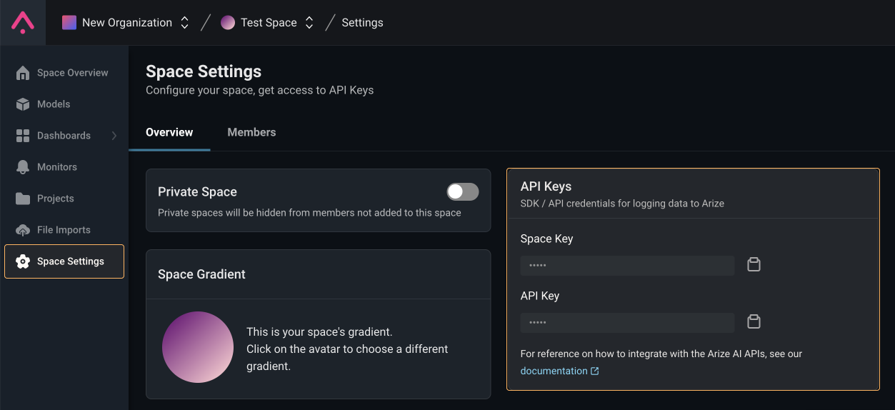
Copy the Arize API_KEY and SPACE_KEY from your Space Settings page (shown below) to the variables in the cell below. We will also be setting up some metadata to use across all logging.

Now that our Arize client is setup, we can log all of our data to the platform. For those interested, here is more detail on how arize.pandas.logger works.

Define the Schema

A schema instance specifies the column names for corresponding data in the dataframe. While we could define different schemas for training and production datasets, the dataframes have the same column names, so the schema will be the same in this instance.

To ingest non-embedding features, it suffices to provide a list of column names that contain the features in our dataframe. Embedding features, however, are a little bit different.

Arize allows you to ingest not only the embedding vector but the raw data associated with that embedding, or a URL link to that raw data. Therefore, up to three columns can be associated with the same embedding object*. To be able to do this, Arize’s SDK provides the EmbeddingColumnNames class, used below.

*NOTE: This is how we refer to the three possible pieces of information that can be sent as embedding objects:

• Embedding vector (required)
• Embedding data (optional): raw text associated with the embedding vector. Not used here.
• Embedding link_to_data (optional): link to the data file (image, audio, …) associated with the embedding vector

Learn more here.

Log Data

Step 5: Confirm Data Is In Arize ✅

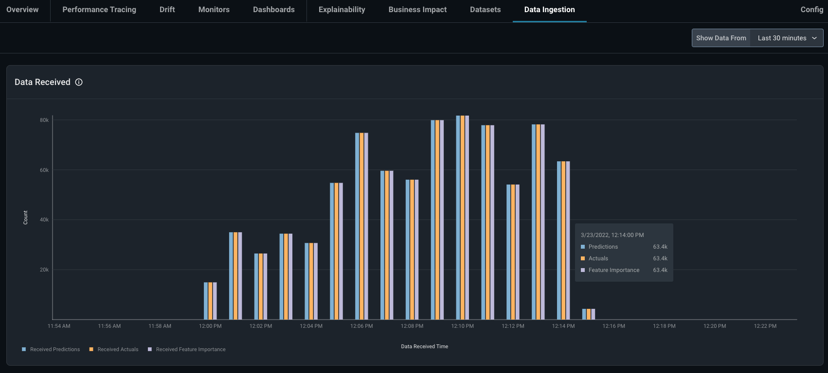
Note that the Arize platform may take around 15 minutes to index embedding data. While the model should appear immediately, the data will not show up until the indexing is complete. Feel free to head over to the Data Ingestion tab for your model to watch the platform work its magic!🔮

You will be able to see the predictions, actuals, and feature importances that have been sent in the last 30 minutes, last day or last week.

An example view of the Data Ingestion tab from a model, when data is sent continuously over 30 minutes, is shown in the image below.

Step 6: Check the Embedding Data In Arize

Now you can see how Arize surfaces the low quality images before your customer notices, troubleshooting the degradation in performance to save you the time and effort.

First, set the baseline to the training set that we logged before.

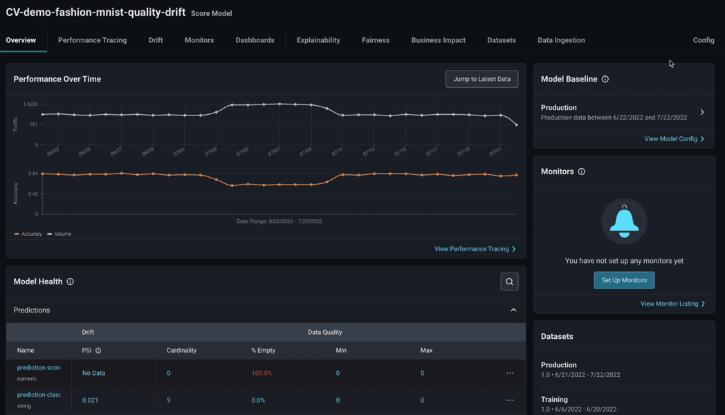
Since your model contains embedding data, you will see it in your Model Overview page.

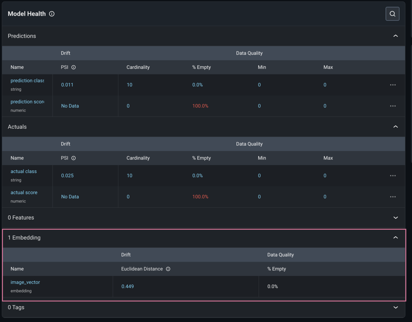
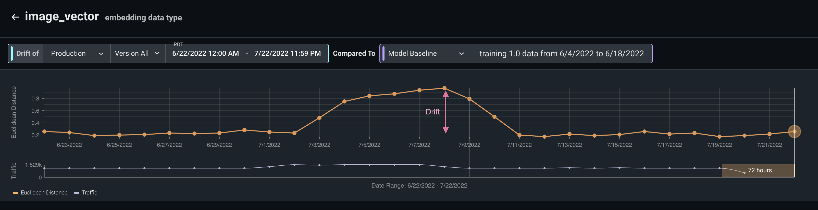
Click on the embedding name or the Euclidean distance value to see how your embedding data is drifting over time. In the picture below, we represent the global euclidean distance between your production set (at different points in time) and the baseline (which we set to be our training set). We can see there is a period of a week where suddenly the distance is remarkably higher. This shows us that during that time image data was sent to our model, it was different than what it was trained on. This is the period of time when the quality of some images is worse.

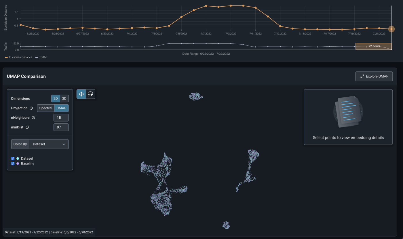
In addition to the drift tracking plot above, you can also leverage a UMAP visualization of your data for the point in time selected. Notice that the production data and our baseline (training) data are superimposed, which is indicative that the model is seeing data in production similar to the data it was trained on.

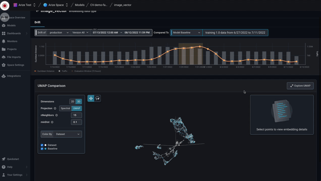
For further inspection, you can select a three dimensional UMAP view and click Explore UMAP to expand the view. With this view, we can interact in 3D with our dataset. We can zoom, rotate, and drag so we can see the areas of our dataset that are most interesting to us. Check out the workflow below:

In the UMAP display, several different color options are available:

• By Dataset: You can see that the coloring has been made to distinguish production data vs baseline data (training in this example). This is specifically useful to detect drift. In this example, we can see that there is some production data far away from any training data, giving an indication of severe dataset drift. We can identify exactly what datapoints our baseline is missing so that we can re-train effectively.
• By Prediction Label: This coloring option gives an insight on how is our model making decisions. Where are the different classes located in the space? Is the model predicting one class in regions where it should be predicting another?
• By Actual Label: This coloring option is great if we want to identify labeling issues. For instance, if inside the orange cloud, we can see a points of other colors, it is a good idea to check and see if the labels are wrong. Further we can use the corrected labels for re-training. This separation is specially difficult when clusters are joined, since both the model and UMAP have trouble separating the data-points.
• By Correctness: This coloring option offers a quick way of identifying where the bulk of your model’s mistakes are placed, giving you an area to pay attention to. In this example, we can see the difference between the red and blue images and almost all the red images have significantly worse quality (e.g. they are rotated and blurred).
• By Confusion Matrix: This coloring option allows you to select a positive class and color the data-points as True Positives, True Negatives, False Positives, False Negatives.
• By Feature: You can identify areas of the space where your model might be underperforming and, by coloring the points by feature, identify patterns at feature level. In other words, you can identify a slice of your data sharing a common feature (or features) that are causing a problem.
• By Prediction Score: You can identify areas where your model is more confident of its predictions and areas where your model struggled more to make a decision.

More coloring options will be added to help you understand and debug your model and dataset.

Final Note

If you want to remove this example model from your account, just click Models -> CV-demo-fashion-mnist-quality-drift -> config -> delete

Conclusion

As more image classification models get deployed into production across a wider array of applications, having monitoring in place to track embedding drift is no longer a nice-to-have — it’s essential, especially in industries like healthcare or self-driving cars where safety is paramount. By taking a few simple steps outlined in this piece, your team can have a more robust and automated way to stay on top of model performance.

Questions? Reach out on the Arize community or book a demo. For additional Colabs, check out the Arize Docs.