
Jensen-Shannon divergence, usually shortened to JS divergence, measures how different two probability distributions are by comparing each of them to their average. Build a mixture distribution M that is halfway between P and Q, measure the KL divergence from each original distribution to that mixture, and average the two results:
JSD(P, Q) = 0.5 * KL(P || M) + 0.5 * KL(Q || M)
where M = 0.5 * (P + Q)
That construction is not a formality. It is what fixes the two properties of KL divergence that make KL awkward to use as a monitoring metric. KL is asymmetric, so the answer changes depending on which distribution you call the reference. KL is also unbounded, and it goes to infinity the moment one distribution puts probability somewhere the other assigns zero. Because the mixture M has support everywhere either P or Q does, neither KL term inside JS divergence can divide by zero.
Build better agents with Arize
Trace, evaluate, and learn. Build agents that work with Arize AX and start tracing your runs today.
Prefer open source? Try Arize Phoenix for self-hosted, open source agent observability.
Key takeaways
- JS divergence is the average KL divergence from each distribution to their midpoint mixture, which makes it symmetric and always finite.
- It is bounded. With a natural log the range is 0 to ln 2; with log base 2 the range is 0 to 1. Two distributions that share nothing sit at the ceiling.
- The square root of JS divergence, known as Jensen-Shannon distance, is a true metric that satisfies the triangle inequality.
- The mixture reference is also its main operational weakness: in a moving-window drift check the reference changes every period, so values from different periods are not directly comparable.
- For continuous variables you have to bin first, and the bin scheme becomes part of the measurement.
How it behaves
Start with two identical distributions and JS divergence is 0. Pull them apart and it rises. Pull them entirely apart, so that no bin holds mass from both, and it stops at its maximum: ln 2 in nats, or exactly 1 if you compute in bits. That ceiling is a genuine tradeoff. It means the metric is easy to reason about and easy to threshold, and it also means the metric cannot tell you that a distribution moved from far away to very far away. Once the supports separate, additional movement is invisible.
Compare that with a transport-based measure such as Wasserstein distance, which keeps climbing as the distributions separate but carries the units of the variable and needs per-feature calibration. Neither is strictly better. JS divergence gives you a normalized, comparable-across-features number with a hard ceiling; transport distance gives you unbounded sensitivity with no natural scale.
The moving-window problem
This is the detail that catches teams out, and it follows directly from the mixture reference.
A typical drift check compares a fixed baseline against a window that slides forward each hour or each day. With JS divergence, the reference is not the baseline: it is the mixture of the baseline and the current window. Since the current window changes every period, the mixture changes every period too. The number you get for Tuesday was computed against a slightly different yardstick than the number you got for Monday.
For a single yes-or-no question, “did this distribution move,” that is usually fine. For a time series of drift values that you want to trend, compare across periods, or alert on with a fixed threshold, it is a real problem. Metrics with a fixed reference, such as population stability index, avoid it because the denominator never moves. There are workarounds, including recomputing the mixture from a frozen baseline pair, but if the primary use case is period-over-period alerting, a fixed-reference metric is usually the cleaner starting point. The broader tradeoffs between drift measures are walked through in when I drift, you drift, we drift.
Binning, and why it matters more than people expect
JS divergence is defined on probability distributions over the same set of outcomes. Categorical features already have those outcomes. Continuous features do not, so you bin them first, and every choice in that binning shows up in the result.
Too few bins and a real shift hides inside a wide bucket. Too many bins and each bucket gets sparse, which makes the estimate noisy and sensitive to sample size. Equal-frequency bins derived from the baseline are a common default because they keep buckets populated on skewed data. Whatever you pick, the bin edges have to be frozen and reused; recomputing edges from each new window measures the binning, not the data.
Empty bins are less dangerous here than with raw KL divergence. Since the mixture always covers both supports, a bin that is populated in one distribution and empty in the other contributes a finite amount rather than an infinity. That is the practical reason JS divergence gets picked over KL for monitoring in the first place.
Where it fits in production monitoring
Distribution distance is one instrument among several. It answers “has the shape of this variable changed” and nothing else. It does not tell you whether the change hurt anything, and it does not tell you what caused it.
In a working setup it sits next to input-side checks such as missingness, type mismatch, and out-of-range rates, and next to outcome-side measurement of latency and error rates. Drift is the leading indicator; the other two tell you whether the lead was real.
For LLM systems the same math applies to two newer kinds of distribution. Categorical eval verdicts, such as the pass and fail labels produced when you run an LLM as a judge, form a distribution over labels that can be compared week over week. High-dimensional embeddings need a reduction step before any binned metric applies, which is the subject of measuring embedding drift.
FAQ
What is the difference between JS divergence and KL divergence?
KL divergence measures the information lost when you use one distribution to approximate another. It is directional, so swapping the arguments changes the answer, and it is infinite whenever the approximating distribution assigns zero probability to an observed outcome. JS divergence averages two KL terms against a shared mixture, which makes it symmetric, bounded, and always finite.
What is Jensen-Shannon distance?
It is the square root of the divergence. Taking the square root produces a quantity that satisfies the triangle inequality, which the raw divergence does not. If you need a true metric, for clustering or nearest-neighbor work, that is the version to reach for.
Does scipy return the divergence or the distance?
The distance. scipy.spatial.distance.jensenshannon takes the square root before returning, and it defaults to a natural log base. If your numbers look smaller than expected, or smaller than a colleague’s on the same data, one of those two defaults is usually the reason.
What JS divergence value should trigger an alert?
There is no portable number even though the metric is bounded, because how far a healthy feature moves between windows depends on your traffic volume and your bin scheme. Compute it across historical windows where you know nothing was wrong, then set the alert above that observed range. Being bounded makes the value comparable across features in the same setup. It does not make it comparable across setups.
Can I use JS divergence on embeddings directly?
Not on the raw vectors. It needs a distribution over a fixed set of outcomes, and a 1,536-dimensional embedding is not that. The usual route is a reduction step first, either projecting to a low-dimensional space and binning, or clustering and comparing cluster frequencies. Either way the reduction becomes part of the measurement and has to be frozen alongside the bin edges.