


SNE vs. t-SNE vs. UMAP: An Evolutionary Guide

Francisco Castillo
Data Scientist / Software Engineer
Introduction
According to multiple estimates, 80% of data generated by businesses today is unstructured data such as text, images, or audio. This data has enormous potential for machine learning applications, but there is some work to be done before it can be used directly. Feature extraction helps extract information from the raw data into embeddings. Embeddings, which we covered in a previous piece, are the backbone of many deep learning models; they are used in GPT-3, DALL·E 2, language models, speech recognition, recommendation systems, and other areas. However, one persistent problem is that it is hard to troubleshoot embeddings and unstructured data today. It is challenging to understand this type of data, let alone recognize new patterns or changes. To help, there are several prominent ways to visualize the embedding representation of the dataset using dimensional reduction techniques. In this piece, we’ll go through three popular dimensionality reduction techniques and their evolution: SNE, t-SNE, and UMAP.
Dimension reduction is a crucial technique in data science that serves as a fundamental tool for both visualization and pre-processing in machine learning. These methods transform high-dimensional data X = {x0, x1, …, xN} into lower-dimensional data Y = {y0, y1, …, yN}, where N represents the number of data points.
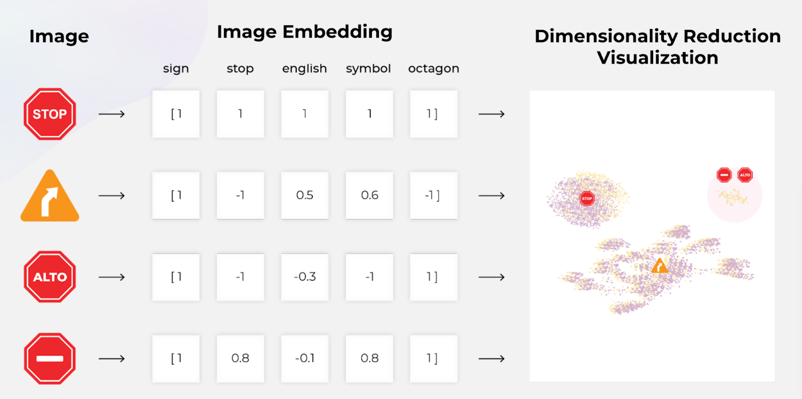
Embeddings, which are often computed in machine learning, are a form of dimension reduction. When dealing with unstructured data, such as images of size WHC (Width, Height, Channels), tokenized language, or audio signals, the input space can be massive. For example, if the input space consists of 1024×1024 images, the input dimensionality exceeds one million. By applying models like ReNet or EfficientNet, embeddings with 1000 dimensions can be extracted, reducing the output space dimensionality by three orders of magnitude. These embeddings are dense, smaller feature vectors that can be referred to as the feature space or embedding space.
Once feature vectors have been generated, further dimensionality reduction is necessary to obtain human-interpretable information. As it is challenging to visualize objects in more than three dimensions, additional tools must be utilized to reduce the dimensionality of the embedding space to two or three dimensions while maintaining relevant structural information.
Dimensionality reduction techniques can be divided into three categories: feature selection, matrix factorization, and neighbor graphs. The latter category, which includes SNE (Stochastic Neighbor Embedding), t-SNE (t-distributed Stochastic Neighbor Embedding), and UMAP (Uniform Manifold Approximation and Projection), will be the focus of this discussion.
SNE, t-SNE, and UMAP are neighbor graphs algorithms that follow a similar process. They begin by computing high-dimensional probabilities p, then low-dimensional probabilities q, followed by the calculation of the cost function C(p,q) by comparing the differences between probabilities. Finally, the cost function is minimized.