As ML practitioners deploy more models into production, the stakes for model performance are higher than ever  –  and the mistakes costlier. It’s well past time for teams to shift to a modern approach to ML troubleshooting. In this content series, we will dive into the evolution of ML teams go through  -  from no monitoring to monitoring to full stack ML observability  – and lessons learned along the way.

Part One: From No Monitoring To Monitoring

To paraphrase a common bit of wisdom, if a machine learning model runs in production and no one is complaining, does it mean the model is perfect? The unfortunate truth is that production models are usually left alone unless they lead to negative business impacts.

Let’s look at an example of what may happen today:

As a machine learning engineer (MLE) for a fintech company, you maintain a fraud-detection model. It has been in production for a week, and you are enjoying your morning coffee when a product manager (PM) urgently complains that the customer support team has seen a significant increase in calls complaining about fraudulent transactions.

This costs the company a fortune in chargeback transactions. The company is spending tens of thousands of dollars every hour, and you have to fix it now.

Gulp. Is it your model? Software engineers tell you that the problem is not on their end.

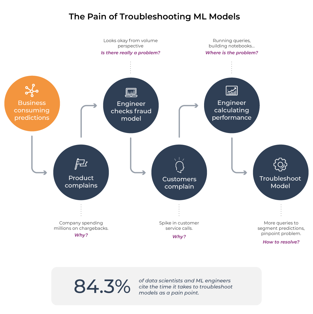
You write a custom query to pull data from logs of the last million predictions that your model has made in the past three days. The query takes some time to run, you export the data, do some minimal preprocessing, import it into a Jupyter notebook, and eventually start calculating relevant metrics for the sample data you pulled.

There doesn’t seem to be a problem in the overall data. Your PM and customers are still complaining, but all you see is maybe a slight increase in fraudulent activity.

More metrics, more analysis, more conversations with others. There’s something going on, it’s just not obvious. So you start digging through the data to find a common pattern on the fraud transactions that the model is missing. You’re writing ad-hoc scripts to slice into the data.

This takes days or weeks of all-consuming effort. Everything else you were working on is now on pause until this issue is resolved because: 1) you know the model the best; and 2) every bad prediction is costing the company revenue.

Eventually you see something odd. If you slice by geographies, California seems to be performing somewhat worse than it did a few days ago. You filter to California and realize some of the merchant IDs belong to scam merchants that your model did not pick up. You retrain your model on these new merchants and save the day.

This example helps us see what it takes to troubleshoot a machine learning model today. It is many times more complex than troubleshooting traditional software. We are shipping AI blind.

There are many monitoring tools and techniques for traditional software engineering—things like Datadog and New Relic—that automatically surface performance problems. But what does monitoring look like for machine learning models?

ML Performance Monitoring

First, let’s make sure we have a definition of what monitoring is: monitoring, at the most basic level, is data about how your systems are performing; it requires that data are made storable, accessible, and displayable in some reasonable way.

What Data Is Needed to Do Performance Monitoring?

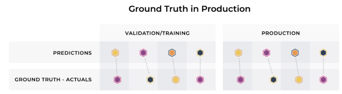
To monitor machine learning models’ performance, you must begin with a prediction and actual.

A model has to make some predictions. This can be predicting the estimated time of arrival (ETA) of when the ride is going to arrive in a ride-sharing app. It can also be what loan amount to give a certain person. A model can predict if it will rain on Thursday. At a fundamental level, this is what machine learning systems do: they use data to make a prediction.

Since what you want is to predict the real world, and you want that prediction to be accurate, it is also useful to look at actuals (also known as ground truth). An actual is the right answer—it is what actually happened in the real world. Your ride arrived in five minutes, or it did rain on Thursday. Without comparison to the actuals, it is very difficult to quantify how the model is performing until your customers complain.

But getting the actuals is not a trivial endeavor. There are four cases here:

1. Quick Actuals: In the easiest case, actuals are surfaced to you for every prediction, and there is a direct link between predictions and actuals, allowing you to directly analyze the performance of your model in production. This can happen in the case of predicting the ETA of your ride, for example. At some point the ride will arrive, and you will know how long that took and whether the actual time matched your prediction.

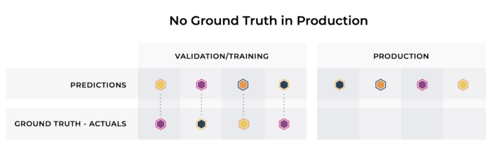
2. Delayed Actuals: In the diagram below, while we see that actuals for the model are eventually determined, they come too late for the desired analysis.

When this actuals delay is small enough, this scenario doesn’t differ too substantially from quick actuals. There is still a reasonable cadence for the model owner to measure performance metrics and update the model accordingly, as one would do in the real-time actuals scenario.

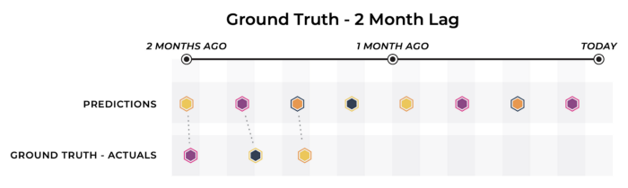
However, in systems where there is a significant delay in receiving the actuals, teams may need to turn to proxy metrics. Proxy metrics are alternative signals that are correlated with the actuals that you’re trying to approximate.

For example, imagine you are using a model to determine which consumers are most likely to default on their credit card debt. A potential proxy metric in this scenario might be the percentage of customers to whom you have lent credit that make a late payment.

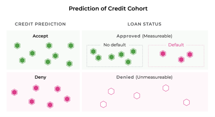
3. Causal Influence on Actuals (Biased Actuals): Not all actuals are created equal. In some cases, teams receive real-time actuals but the model’s predictions have substantially affected the outcome. To take a lending example, when you decide to give loans to certain applicants, you will receive actuals on those applicants but not those you rejected. You will never know, therefore, whether your model accurately predicted that the rejected applicants would default.

4. No Actuals: Having no actuals to connect back to model performance is the worst-case scenario for a modeling team. One way to acquire ground truth data is to hire human annotators or labellers. Monitoring drift in the output predictions can also be used to signal aberrant model behavior even when no actuals are present.

For a deeper dive on these scenarios, see our “Playbook To Monitor Your Model Performance In Production.”

Gathering your predictions and your actuals is the first step. But in order to do any meaningful monitoring, you need to have a formula for comparing your predictions and your actuals — you need the right metric.

What Are the Right Metrics for My Model?

The correct metric to monitor for any model depends on your model’s use case. Let’s look at some examples.

Fraud

A fraud model is particularly hard to assess with simple measures of accuracy since the dataset is extremely unbalanced (a great majority of transactions are not fraudulent). Instead, we can measure:

• Recall, or what portion of fraud examples your model identified that are true positives.
• False negative rate measures fraud that a model failed to predict accurately. It is a key performance indicator since it’s the most expensive to organizations in terms of direct financial losses, resulting in chargebacks and other stolen funds.
• False positive rate — or the rate at which a model predicts fraud for a transaction that is not actually fraudulent — is also important because inconveniencing customers has its own indirect costs, whether it’s in healthcare where a patient’s claim is denied or in consumer credit where a customer gets delayed buying groceries.

Demand Forecasting

Demand forecasting predicts customer demand over a given time period. For example, an online retailer selling computer cases might need to forecast demand to make sure that they can meet customer needs and not buy too much inventory. Like other time-series forecasting models, it is best described by metrics like ME, MAE, MAPE, and MSE.

• Mean error (ME) is average historical error (bias). A positive value signifies an overprediction, while a negative value means underprediction. While mean error isn’t typically the loss function that models optimize for in training, the fact that it measures bias is often valuable for monitoring business impact.
• Mean absolute error (MAE) is the absolute value difference between a model’s predictions and actuals, averaged out across the dataset. It’s a great first glance at model performance since it isn’t skewed by extreme errors of a few predictions.
• Mean absolute percentage error (MAPE) measures the average magnitude of error produced by a model. It’s one of the more common metrics of model prediction accuracy.
• Mean squared error (MSE) is the difference between the model’s predictions and actuals, squared and averaged out across the dataset. MSE is used to check how close the predicted values are to the actual values. As with root mean square error (RMSE), this measure gives higher weight to large errors and therefore may be useful in cases where a business might want to heavily penalize large errors or outliers.

Other Use Cases

From click-through rate to lifetime value models, there are many machine learning use cases and associated model metrics. For additional reference, see Arize’s model monitoring use cases.

What Are the Right Thresholds?

So now you have your metric, and you’re faced with a new problem: how good is good enough? What is a good accuracy rate? Is my false negative rate too high? What is considered a good RMSE?

Absolute measures are very difficult to define. Instead, machine learning practitioners must rely on relative metrics. In particular, you must determine a baseline performance. While you are training the model, your baseline could be an older model you have productized, a state-of-the-art model from literature, or human performance. But once the model is in production, it becomes its own benchmark. If you have a three percent false negative rate on day one and then a 10% false negative rate today, you should wake up your engineers!

Often, initial performance is not what is actually used; instead, you can use a rolling 30-day performance.

When the model shifts significantly (a standard deviation or more), an alert must be triggered. This should be an automated setup based on a baseline dataset so that you can be alerted proactively.

Conclusion & What’s Next

Machine learning models have been adopted quickly over the last decade, solving very complex problems with large business impacts. Machine learning systems are usually built on top of data pipelines and other complex engineering systems that feed the models the data needed to make predictions. But predictions are only the beginning. To run these systems reliably in production, you need performance monitoring to continuously assess your model’s accuracy and quality.

Of course, monitoring alone is not enough. If you’re at this stage, you might get an alert before your customers complain about an uptick in fraudulent transactions but you still don’t know how to easily go fix it. In part two of this blog series, we will cover a modern and less painful approach to assessing and troubleshooting model performance: full stack ML observability with ML performance tracing.