
LIME, or Local Interpretable Model-Agnostic Explanations, is an explainability method that attempts to provide local ML explainability. At a high level, LIME attempts to understand how perturbations in a model’s inputs affect the end prediction of the model. Since it makes no assumptions about how the model reaches the prediction, it can be used with any model architecture, hence the model-agnostic part of LIME.
The LIME explainability approach takes a single input, perturbs features around that instance, observes how predictions change, and fits a simple interpretable model (usually a linear model) to those neighborhood samples. The coefficients become feature importances for that one prediction. You get a local story: which inputs pushed this row toward class A instead of class B.
Key takeaways
- LIME explains one prediction at a time by approximating the opaque model locally with a simpler surrogate.
- It is model-agnostic: same workflow for trees, neural nets, and API-backed scorers if you can query predictions.
- Explanations depend on how you define neighborhoods, especially for text, images, and correlated tabular features.
- LIME is local, not global. A feature important for row 42 may barely matter elsewhere.
- SHAP values offer a different attribution framework with stronger axioms but higher compute cost on some models.
How LIME works step by step
Pick an instance x you want to explain. Sample perturbed versions x' by flipping, masking, or noising features according to a perturbation policy:
- Generate neighborhood. Tabular: toggle binarized features or add Gaussian noise. Text: remove or hide word subsets. Images: superpixel masks.
- Label with the original model. Query
f(x')for each perturbation. You only need prediction access, not gradients. - Weight by proximity. Perturbations closer to
xcount more in the fit. - Fit an interpretable surrogate. Weighted linear regression (or sparse linear model) predicts
f(x')from perturbation indicators. - Read coefficients. Large positive weights push toward the predicted class; negative weights push away.
The surrogate is intentionally wrong globally. It only needs to match f near x.
from lime.lime_tabular import LimeTabularExplainer
explainer = LimeTabularExplainer(X_train, mode="classification")
exp = explainer.explain_instance(x, predict_fn, num_features=10)
Local vs global explainability
Local methods answer: “Why this prediction for this customer?” Global methods answer: “Which features matter overall?”
LIME is local. Running it on many rows and averaging coefficients is a heuristic global view, not a guaranteed summary. Correlated features swap importance between runs unless you regularize or group them.
For regulatory or debugging workflows, local explanations pair with slice analysis. If LIME cites account_age for ten disputed declines, you inspect those rows together instead of trusting one heatmap.
Model-agnostic benefits and costs
Benefits:
- Same API for scikit-learn pipelines, XGBoost, PyTorch, or remote endpoints.
- Useful when internal model structure is unknown (vendor API, legacy binary).
- Fast to prototype on tabular rows with modest feature count.
Costs:
- Perturbation design is the whole game. Bad neighborhoods produce confident but false stories.
- Stability varies. Re-run LIME with different seeds and features may shuffle ranks.
- High-dimensional sparse inputs need many samples for faithful local fits.
Model-agnostic does not mean assumption-free. You still choose distance metrics, discretization bins, and kernel width.
LIME vs SHAP and other attribution methods
SHAP values come from cooperative game theory and satisfy additivity: feature attributions sum to the difference between the prediction and a baseline expectation. TreeSHAP computes exact values efficiently for tree ensembles. Kernel SHAP generalizes like LIME but with Shapley-weighted samples.
Practical differences teams notice:
- Stability. SHAP with fixed background data can be more reproducible than LIME when perturbations are noisy.
- Compute. Explaining many rows with Kernel SHAP is slow. LIME can be slow too on high-dimensional text unless sampling is tuned.
- Linear models. For truly linear scorers, coefficients already are global explanations. LIME and SHAP add little.
Integrated gradients and gradient-based methods need differentiable models but scale differently. Pick LIME when you only have prediction API access and feature count is manageable.
Failure modes to expect
Correlated features. LIME may split credit between collinear income columns arbitrarily. Group features, use domain bundles, or prefer methods that handle correlation explicitly.
Text and image perturbations. Removing random words may leave ungrammatical strings far from the manifold of real inputs. The local model explains the surrogate task, not always the human notion of “why.”
Class imbalance and sharp thresholds. Near decision boundaries, tiny input changes flip labels. LIME neighborhoods straddle the boundary and coefficients swing.
Wrong trust in production. An explanation is not causality. Use LIME to generate hypotheses, then validate with ablation tests or labeled counterfactuals.
When drift appears, local explanations from an old model version mislead. Tie explanation jobs to registered model IDs and re-run after retrain. Model and concept drift monitoring should trigger refreshed explainability samples on affected slices, not one static dashboard from launch day.
When teams still use LIME
Prototypes and incident reviews: explain ten failing rows before you inspect logs in detail.
Vendor and legacy models: no weight access, but JSON in and score out.
Teaching and stakeholder communication: a short list of weighted features beats a dense SHAP beeswarm for some audiences.
Hybrid workflows: LIME for quick triage, SHAP or tree native importances for regression tests before release.
For vision models, LIME superpixel maps remain a teaching tool even when production teams rely on other monitors. Shipping image classification with confidence includes calibration and slice metrics; local attributions supplement where the model fires on the wrong object class.
Store explanation configs (kernel width, sample count, feature grouping) in AI model lifecycle management metadata so auditors know how charts were produced.
FAQ
What does LIME stand for?
Local Interpretable Model-Agnostic Explanations. Local: one instance at a time. Interpretable: surrogate is simple, usually linear. Model-agnostic: only prediction access required.
Is LIME global or local?
Local. Each explanation applies to one input neighborhood. Aggregate carefully if you need global importance.
Can LIME explain LLM outputs?
Only through a tabular or token perturbation wrapper you define. Explaining free-form text generation needs careful perturbation design and is easy to misread. Many LLM teams prefer prompt-level evals and traced tool calls over LIME on raw strings.
How is LIME different from SHAP?
Both can use perturbations, but SHAP targets Shapley values with additivity guarantees. LIME fits a weighted local surrogate with more freedom in kernel and sampling. SHAP is often more reproducible; LIME can be faster to wire up for quick probes.
How many perturbations does LIME need?
Enough that the local surrogate fits the original model’s responses in the neighborhood. Tabular problems with tens of features may need thousands of samples; low-dimensional cases need fewer. Validate stability by re-running and checking top features.