
Current distribution refers to the statistical distribution, or shape, of the dataset being generated by a machine learning model in production. Distribution of datasets in machine learning models are represented in the form of functions that show the relationships between the various observations, visually presented in the form of curves or graphs. In monitoring, “current” almost always means a rolling production window you compare against a frozen reference distribution from training or an earlier stable period.
Build better agents with Arize
Trace, evaluate, and learn. Build agents that work with Arize AX and start tracing your runs today.
Prefer open source? Try Arize Phoenix for self-hosted, open source agent observability.
Key takeaways
- Current distribution describes how values fall across bins or categories in live traffic right now.
- Compare current to reference distributions to detect data drift, score shift, and calibration changes.
- Histograms, ECDFs, and PSI tables are common views; bin definitions must stay stable over time.
- Monitor both feature inputs and model outputs (scores, embeddings, predicted classes).
- Empty or sparse bins in current data inflate drift statistics; apply smoothing and minimum count rules.
What gets measured
Input features. Numeric columns (amounts, counts, durations), categorical levels (country, device), and text-derived signals (length, language id).
Model outputs. Predicted probabilities, logits, embedding norms, and argmax labels.
Metadata tags. Not always model inputs but useful for slicing current distributions by cohort.
Each metric you chart should declare its aggregation window (hourly, daily, weekly) and whether nulls are included.
Document the filter predicates used to build each chart: model version, route, tenant, and environment tags. Without that metadata, two engineers can compute different “current” curves from the same raw log store and argue past each other during incidents.
Reference versus current
Monitoring stacks store a reference distribution from training, validation, or a golden month of production. On each schedule tick they histogram current production rows with identical bin edges.
Population Stability Index (PSI) and similar scores summarize how far current mass moved relative to reference. Large moves on important features rank ahead of cosmetic ones for investigation.
If you recompute bin edges every week on current data alone, you lose comparability. Fix edges in model artifacts.
Choose reference windows that match the decision your alert triggers. A training snapshot is strict for long-term studies; a rolling prior-week reference catches sudden step changes faster after deploys or outages.
Visualization practices
Overlay reference and current histograms for quick eyeballing. Use logarithmic y-axis when tails are heavy.
For high-cardinality strings, collapse rare levels into an “other” bucket before comparing.
Embedding spaces use dimensionality reduction (UMAP, PCA) on sample batches; compare cluster proportions rather than raw coordinates, which are not stable across runs.
Empirical CDF plots help when means hide quantile movement. A unchanged average with a longer tail in current data still changes rank-based model behavior.
Operational use
Current distribution dashboards answer: “Did today’s traffic look like what we trained on?” Spikes in missing values, new category levels, or score compression often precede metric degradation.
Pair distribution charts with performance slices. A feature whose current distribution shifted may still be harmless if labels are unchanged, or it may drive false positives in fraud.
Use shadow traffic before major releases to compare current shadow score distributions to production reference without affecting users.
Workflow posts on model, concept, and data drift explain tying distribution alerts to label eval backfills.
Lifecycle documentation in AI model lifecycle management covers where to store reference snapshots alongside model versions.
For text models, token length and language mix in current inputs affect quality; NLP monitoring examples in NLP sentiment classification monitoring show cohort views that complement global histograms.
Failure modes
Sample bias. Logging only successful requests skews current distributions.
Clock skew. Misaligned windows compare partial days to full reference weeks.
Too-granular bins. Sparse counts create noisy PSI without real shift.
Ignoring output drift. Input stability with score drift still breaks calibration and threshold policies.
FAQ
How is current distribution different from reference distribution?
Reference is the baseline you trust (training or stable past). Current is production traffic in the evaluation window you are inspecting now.
How often should I refresh the reference?
When you intentionally retrain or after a verified stable regime change. Ad hoc refreshes erase history needed for incident postmortems.
Should I monitor embeddings as distributions?
Yes, via projection samples, cluster counts, or distance to centroids. Raw high-dimensional histograms per dimension are usually too noisy.
What sample size do I need?
Enough rows per bin for stable percentages. Low-volume models may need multi-week windows; high-volume can use hourly with caution on noise.
Can current output distribution shift without data drift?
Yes, when the model version changes, thresholds move, or concept drift alters labels while inputs look similar.