


https://storage.googleapis.com/arize-phoenix-assets/assets/images/phoenix-docs-images/gc.ico

Google Colab

colab.research.google.com
When a new model tops MMLU, GPQA, or the latest leaderboard, it’s tempting to assume it’s the right choice for your application. It usually isn’t — at least not for the reason you think. Public benchmarks measure generic capabilities on generic data with a generic metric: broad academic knowledge, scored as multiple-choice accuracy, averaged over thousands of questions that look nothing like your production traffic. Your task is narrow and specific. You aren’t asking the model trivia — you’re asking it to pull a handful of exact fields out of a customer email, every time, in a schema your downstream code can parse. A model that wins MMLU by two points can lose your task by twenty, because:
  • The data is different — your inputs are your customers’ emails, not exam questions.
  • The metric is different — you care whether the due_date field is exactly right, not whether the prose sounds smart.
  • The failure modes are different — a confident, plausible-sounding wrong answer is worse for you than an “I don’t know,” the opposite of what a knowledge benchmark rewards.
The only benchmark that predicts how a model performs on your task is a benchmark built from your task — and Phoenix experiments are exactly that harness. This cookbook builds one for an email text-extraction service and uses it to compare two models fairly. This cookbook shows examples of:
  • Building a small domain dataset of emails + correct extractions — your benchmark, not a public one
  • Defining an extraction task with a fixed schema and prompt, parameterized only by model
  • Defining two evaluators — string similarity and field-level accuracy — and seeing how they can rank the models differently
  • Running the same harness across gpt-5.4-mini and the flagship gpt-5.5 and comparing them fairly

What makes a benchmark trustworthy

Before trusting any number — public or your own — ask whether the benchmark behind it has these four properties:
  1. Representative data. The examples are drawn from your real inputs, covering the cases you actually see (including the messy and ambiguous ones), not a clean toy sample.
  2. A metric that measures what you care about. The score moves when the output gets better for your purpose and stays flat when it doesn’t. The wrong metric can rank a worse model first — we’ll show exactly this below.
  3. Enough examples to be stable. Two examples can’t distinguish two models; the score has to be more signal than noise.
  4. Reproducible and fair. Every model is judged on the same dataset, with the same metric, under the same prompt — so a difference in the score reflects a difference in the model, not the setup.
A Phoenix experiment is this harness: a fixed dataset, a task you vary, and one or more evaluators. Hold the dataset and evaluators constant, swap only the model, and the comparison is fair by construction.

Notebook Walkthrough

We will go through key code snippets on this page. To follow the full tutorial, check out the full notebook. After configuring tracing with phoenix.otel.register(...) and instrumenting OpenAI, we build a small hand-labeled dataset, define a model-parameterized extraction task, score it two ways, and run the same harness across two models.

Set up tracing

Register a tracer provider so every extraction call shows up as a span in Phoenix — the experiment results link back to the exact calls that produced them. auto_instrument=True activates the installed OpenInference instrumentors (here, OpenAI), so there’s no need to call OpenAIInstrumentor().instrument(...) yourself. Use AsyncClient because the experiment task makes network-bound LLM calls.
from phoenix.client import AsyncClient
from phoenix.otel import register

register(project_name="email-extraction-eval-harness", auto_instrument=True)

px_client = AsyncClient()

Build a domain dataset

This is the part public benchmarks can’t do for you. Hand-label a handful of emails the way your service actually sees them — a meeting request, an invoice, a support escalation — each paired with the exact structured output you want back. In production you’d build this from real traffic (export traces from Phoenix, sample, and label); here we inline a small set so the example is self-contained. The mix of free-text fields (summary) and categorical fields (category, due_date) is deliberate: it’s what lets two reasonable metrics disagree later.
This is a demonstration harness. Eight examples is enough to show the workflow, not to draw stable conclusions (recall property 3 above). A production harness needs a larger, representative sample drawn from your real traffic before you’d trust the ranking.
from datetime import datetime, timezone

import pandas as pd
from phoenix.client.utils.config import get_base_url

# EMAILS = [{"email": "...", "expected": {"sender": ..., "category": ..., "summary": ...,
#            "action_required": ..., "due_date": ...}}, ...]  — see the notebook for the full set.

# Flatten each example's expected extraction into top-level columns, so the dataset's
# output IS the extraction dict the evaluators compare against — not a nested wrapper.
rows = [{"email": e["email"], **e["expected"]} for e in EMAILS]
df = pd.DataFrame(rows)
OUTPUT_KEYS = ["sender", "category", "summary", "action_required", "due_date"]

dataset = await px_client.datasets.create_dataset(
    name=f"email-extraction-{datetime.now(timezone.utc):%Y%m%d-%H%M%S}",
    dataframe=df,
    input_keys=["email"],
    output_keys=OUTPUT_KEYS,
)

# Print a link straight to the dataset so you can eyeball the examples you just uploaded.
base_url = str(get_base_url()).rstrip("/")
print(f"View the dataset in Phoenix: {base_url}/datasets/{dataset.id}/examples")

Define the extraction task

The task is what we hold almost constant: the same schema, the same prompt, the same parsing — only the model changes. Using structured outputs forces every model to return the exact same shape, so the comparison is about extraction quality rather than formatting luck.
make_task(model) returns a task function bound to one model. The experiment calls it once per dataset example; the input it receives is that example’s input dict ({"email": ...}).
from typing import Literal

from openai import AsyncOpenAI
from pydantic import BaseModel

openai_client = AsyncOpenAI()


class EmailExtraction(BaseModel):
    sender: str
    category: Literal["meeting", "invoice", "support_request", "sales", "internal_update"]
    summary: str
    action_required: bool
    due_date: str  # ISO date (YYYY-MM-DD) or the literal string "none"


PROMPT = (
    "Extract structured fields from the email below. "
    "sender must be the sender's email address. "
    "category must be one of: meeting, invoice, support_request, sales, internal_update. "
    'due_date must be an ISO date (YYYY-MM-DD) or the literal string "none". '
    "action_required is true if the email asks the recipient to do something.\n\nEMAIL:\n{email}"
)


def make_task(model: str):
    async def task(input) -> dict:
        response = await openai_client.beta.chat.completions.parse(
            model=model,
            messages=[{"role": "user", "content": PROMPT.format(email=input["email"])}],
            response_format=EmailExtraction,
            # Leave temperature at the model default — a fair comparison varies only the
            # model, and the newest models accept only their default sampling settings.
        )
        return response.choices[0].message.parsed.model_dump()

    return task

Choose metrics that measure what you care about

This is where benchmarks quietly lie. Score the same outputs two ways:
  • jaro_winkler — string similarity on the free-text summary field. Cheap and forgiving — the kind of “looks about right” metric people reach for first — and the right tool for a summary, which can be correct while worded differently.
  • field_accuracy — the fraction of the operational fields (sender, category, action_required, due_date) that match exactly (case-insensitive). This is what downstream code depends on: a due_date that’s “close” is still a wrong date. summary is deliberately left out — exact-matching a summary would punish good extractions for harmless rewording.
The two metrics measure genuinely different things, so they can rank the models differently: a model might write better summaries (higher jaro_winkler) while miscategorizing more emails (lower field_accuracy), or vice versa. When they disagree, the metric that should decide is the one tied to your downstream needs — here, field_accuracy.
import jarowinkler

# jaro_winkler scores only the free-text summary; field_accuracy judges only the
# operational fields downstream code actually depends on. The two never overlap,
# so they can move independently.
OPERATIONAL_FIELDS = ["sender", "category", "action_required", "due_date"]


def jaro_winkler(output, expected) -> float:
    """Forgiving string similarity on the free-text summary (reworded-but-correct still scores high)."""
    return jarowinkler.jarowinkler_similarity(
        str(output.get("summary", "")),
        str(expected["summary"]),
    )


def field_accuracy(output, expected) -> float:
    """Fraction of OPERATIONAL fields that match exactly (case-insensitive)."""
    matches = sum(
        1
        for k in OPERATIONAL_FIELDS
        if str(output.get(k)).strip().lower() == str(expected[k]).strip().lower()
    )
    return matches / len(OPERATIONAL_FIELDS)


EVALUATORS = [jaro_winkler, field_accuracy]
The two metrics can rank the same outputs in opposite order. Made deterministic — two candidate extractions for one invoice email: one with the right operational fields but a reworded summary, one that looks almost identical but has the due_date off by a day:
expected = {
    "sender": "billing@cloudhost.com", "category": "invoice", "action_required": True,
    "due_date": "2025-06-30", "summary": "CloudHost invoice #88231 for $4,200 is due June 30.",
}
# A: every operational field right, but the summary is fully reworded (harmless).
candidate_a = {**expected, "summary": "Please arrange payment for the recent cloud hosting charges before the close of the current billing period."}
# B: summary identical, but the due_date is off by a day.
candidate_b = {**expected, "due_date": "2025-07-01"}

# field_accuracy prefers A (1.000 vs 0.750 — every operational field correct).
# jaro_winkler prefers B (1.000 vs 0.461 — its summary is word-for-word identical).
# But B's one-day date slip is exactly what breaks downstream code: same outputs,
# opposite rankings, and the strict metric is the one that's right.

Run the same harness across models

Same dataset, same evaluators, same prompt — change only the model argument. That’s what makes this a fair comparison instead of an anecdote.
experiment_full = await px_client.experiments.run_experiment(
    dataset=dataset, task=make_task("gpt-5.5"), evaluators=EVALUATORS, experiment_name="gpt-5.5"
)
experiment_mini = await px_client.experiments.run_experiment(
    dataset=dataset, task=make_task("gpt-5.4-mini"), evaluators=EVALUATORS, experiment_name="gpt-5.4-mini"
)

Compare fairly

Phoenix prints a per-experiment summary and lets you compare both runs example-by-example in the UI. Rolling the scores up per metric makes the disagreement explicit:
from collections import defaultdict


def average_scores(experiment) -> dict:
    sums, counts = defaultdict(float), defaultdict(int)
    for run in experiment["evaluation_runs"]:
        result = run.result
        if result and result.get("score") is not None:
            sums[run.name] += result["score"]
            counts[run.name] += 1
    return {name: sums[name] / counts[name] for name in sums}
With only eight examples the two models may or may not separate cleanly on a given run — that’s exactly why you look rather than assume. The lesson holds regardless: if the two metrics rank the models differently, the public-leaderboard instinct (“just take the higher-scoring model”) could have led you to the wrong choice — which model is “better” depends on the metric, and the metric that should win is the one that reflects your downstream needs (here, field_accuracy). If they agree, you now have evidence grounded in your data and your metric. Either way, you trust the result because you built the harness.

Reading the results in Phoenix

Open the dataset’s Experiments tab to see the runs side by side. Each experiment is a row; each evaluator becomes its own score column (so field_accuracy sits next to jaro_winkler), alongside operational columns — average latency, cost, and error rate — that matter for a real model choice but never show up on a public leaderboard.
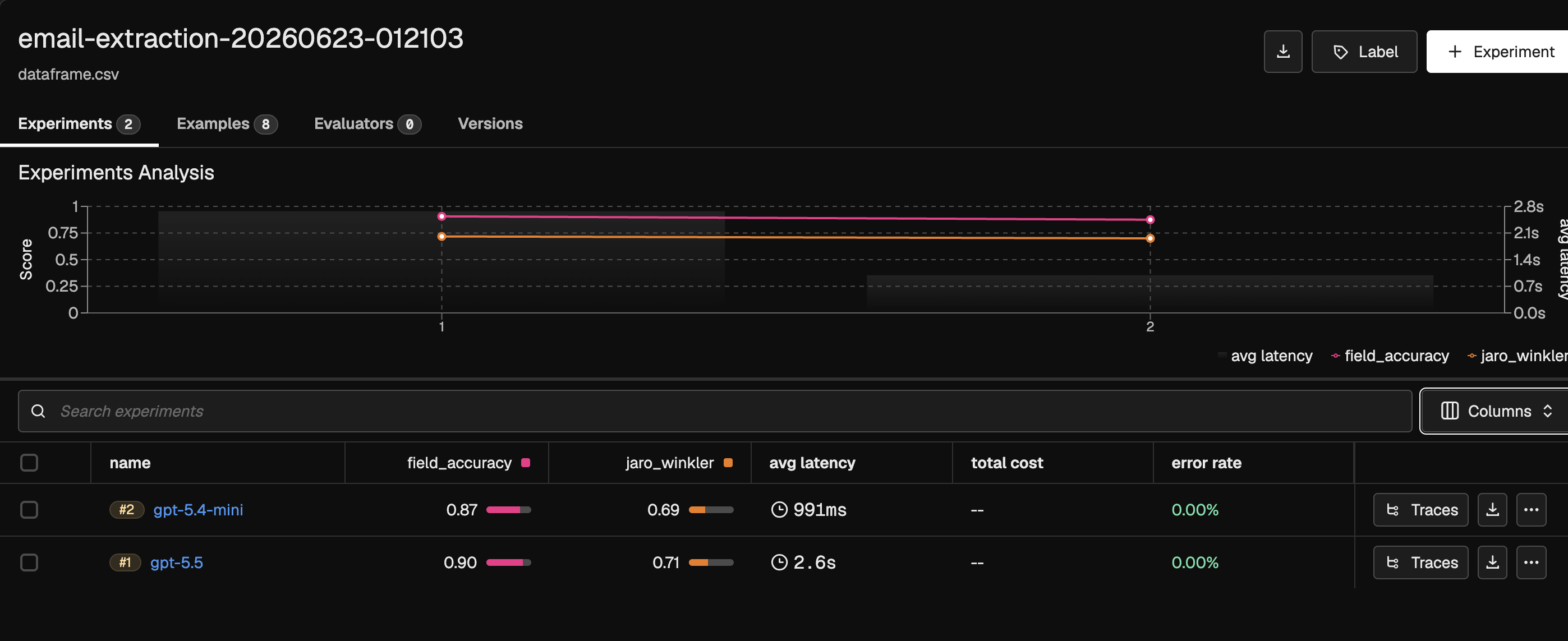
Comparing the gpt-5.5 and gpt-5.4-mini experiments in Phoenix — field_accuracy, jaro_winkler, latency, cost, and error rate side by side.
The two metrics can rank the models differently — a model that writes better summaries (higher jaro_winkler) might still miscategorize more emails (lower field_accuracy), or vice versa. When they disagree, sort by the metric tied to your downstream needs (field_accuracy) rather than the forgiving one, and click any row to drop into the example-level view: the input email, the model’s extraction, and each evaluator’s score for that single example. That’s where you see why one model wins — a due_date the model dropped, a sender it over-captured — instead of trusting an aggregate.
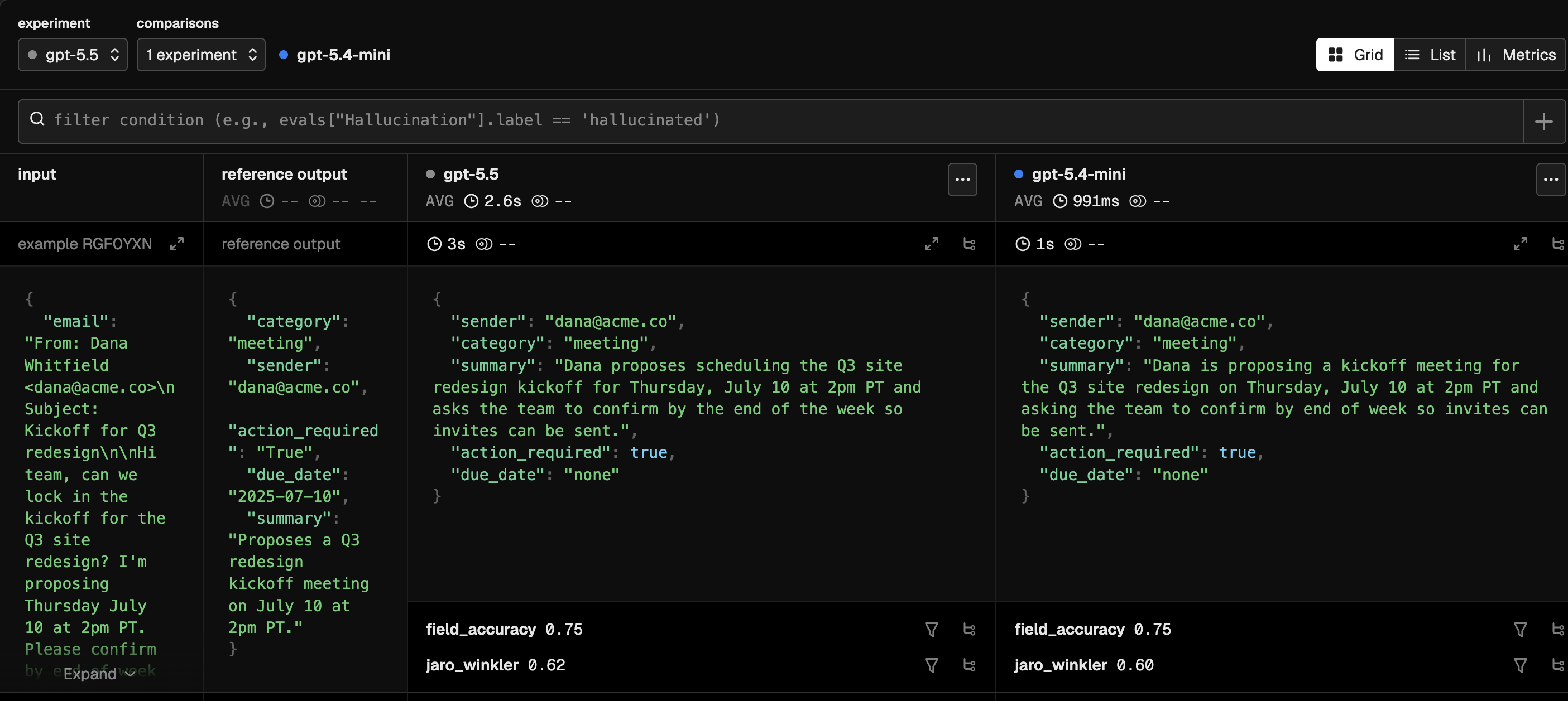
The example-level compare view in Phoenix: the input email, the reference extraction, and the model's output with per-example field_accuracy and jaro_winkler scores.

Where to go next

The harness is reusable — everything below holds the dataset and evaluators constant and changes one thing at a time, so each comparison stays fair:
  • Iterate the prompt. Vary PROMPT instead of model to find the wording that extracts most reliably.
  • Add models and providers. Drop another model name — or another provider’s client — into make_task and rerun. The leaderboard ranking rarely survives contact with your task.
  • Grow the dataset. Move from eight inline examples to a representative sample exported from your real traffic, so the scores become stable enough to trust (property 3).
  • Make it a standing benchmark. Rerun the same harness on every model upgrade or prompt change to catch regressions before they reach production.

Takeaway

A public benchmark tells you how a model does on someone else’s task, with someone else’s metric. That number rarely transfers to production. The fix isn’t a better leaderboard — it’s a small, trustworthy harness of your own:
  • Representative data — a dataset built from your real inputs.
  • A metric that measures what you care about — and the discipline to notice when a convenient metric (string similarity) disagrees with the real one (field accuracy).
  • Enough examples to make the score stable.
  • A fair, repeatable setup — same dataset, same evaluators, same prompt; vary only the model. (Run-to-run sampling adds a little noise, but with the dataset, prompt, and evaluators held fixed, a difference in score still traces to the model — that’s the point, not bit-for-bit reproducibility.)
A Phoenix experiment gives you all four. Once you have it, comparing models — or prompts, or providers — is just swapping one argument and reading a number you can actually defend.