Benchmarking Evaluation of LLM Retrieval Augmented Generation

This piece is co-authored by Evan Jolley and Erick Siavichay

In a search and retrieval system, a knowledge base is a source of structured data that a large language model (LLM) can tap into to answer queries, make recommendations, generate content, or other tasks. The knowledge base serves as the reference against which search queries are matched and results retrieved. Without the use of a knowledge base, an LLM operates in a constrained environment. While it can generate coherent text based on pre-existing patterns learned during training, it lacks the capacity to access, recall, or utilize specific pieces of information that are not embedded in its training data.

The advent of an incredible breadth of retrieval approaches along with LLMs who can take advantage of those systems has led to a lot of options for AI engineers to tinker with.

With so many possibilities, what actually works? There are new retrieval approaches popping up every day, with anecdotal evidence that some are better than others but few hard numbers about what people should do with their own data. We set up a RAG system to put these variables to the test.

Experiment Context and Overview of Findings

The primary source of data in our experiment is Arize AI’s product documentation, which is chunked and seeded into a vector store. With a set of potential user questions ranging from general inquiries to specific questions about product features, the system produces outputs based on these queries which are in turn evaluated by the open source Phoenix LLM evals library. Key metrics include:

• Precision of Context Retrieved: How relevant and accurate is the information retrieved from the vector store when posed with a query?
• Accuracy of the LLM Output: Post-retrieval, how coherent and contextually accurate are the chatbot’s responses?
• System Latency: Given that response time can significantly impact user experience, how long does the system take to provide output?

This writeup is an early attempt to add a rigorous testing layer to the latest LLM retrieval solutions. It includes both results and test scripts (notebook with these scripts to see an example of how they are run here) to parameterize retrieval on your own docs, determine performance with LLM evaluations and provide a repeatable framework to reproduce results.

The following takeaways are based on testing on the aforementioned product documentation (each is explored in greater depth below).

Chunk Sizes

Generally, chunk sizes of 300/500 tokens seem to a good target; going bigger has negative results.

Retrieval Algorithms

Retrieval algorithms have a latency and value tradeoff - if you have user interactivity requirements, you are likely better off sticking to the vanilla, simple approach. If accuracy is paramount and time does not matter, the fancier retrieval algorithms such as re-ranking or HyDE can markedly improve precision.

On K size

4–6 (or even lower) seems optimal trade off for performance and results. Given latency considerations, 4 might be the best bet.

Latency

Latency scales quickly with increasing K and retrieval method complexity.

Your Mileage May Vary

As always, it’s crucial to conduct your own experiments to determine the best parameters for your specific use case.

Parameters: Optimizing RAG Settings

What Is “K”

One of the most important parameters to consider is K, the number of returned chunks from the vector store. The vector store returns chunks of context, and those contexts can be returned a number at a time in order of similarity.

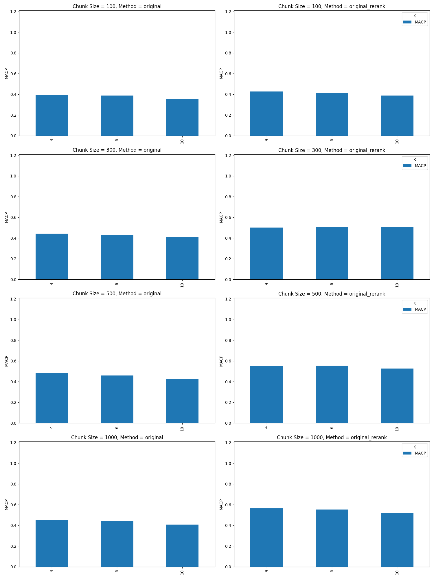
The above figure shows a sweep of K sizes 4, 5, and 6 across two retrieval approaches. For example, in the case K=6, six chunks of text are returned of that specific token size.

It is expected that as you increase K for a fixed size set of relevant documents, that precision at K will drop. The above results do imply we are returning more relevant documents as we increase K.

Precision at k is the number of relevant items in the top k divided by k. If there is a fixed number of relevant items, and k increases while the number of relevant items in the top k remains constant or increases more slowly than k, then Precision at k will decrease.

Mean Reciprocal Rank of Retrieval

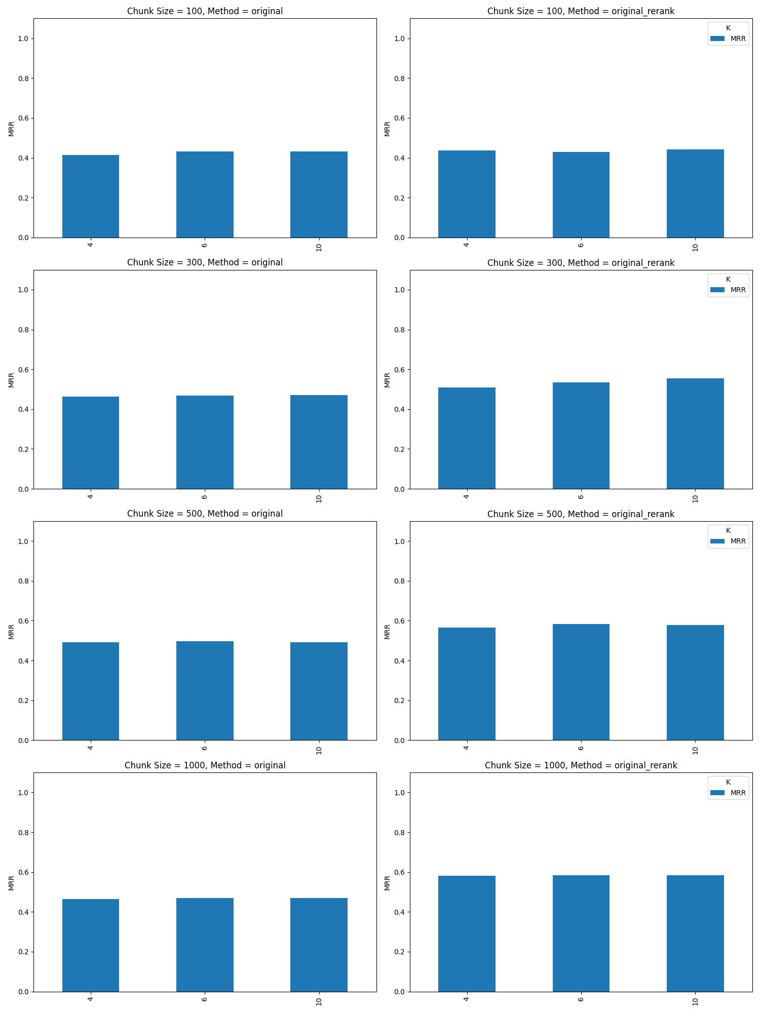
Another way we can look at retrieval results is look at mean reciprocal rank (MRR), included below:

Another way we can look at retrieval results is look at mean reciprocal rank (MRR), included below:
The MRR mimics the retrieval results of the precision @k, about equal retrieval results with a slight edge to chunk = 500/1000 and k=4.

It’s worth noting that our dataset has a number of cases built where there are questions the system can’t answer. Zero retrieval in the dataset is expected for those questions. We have plots in the appendix removes those zero retrieval questions. It skews the numbers lower for all metrics but represents a real world scenario we see in practice.

At first glance the above results imply we should consider as high a K as possible - but we will find looking at other numbers, we will find the lower K of 4/6 a better choice.

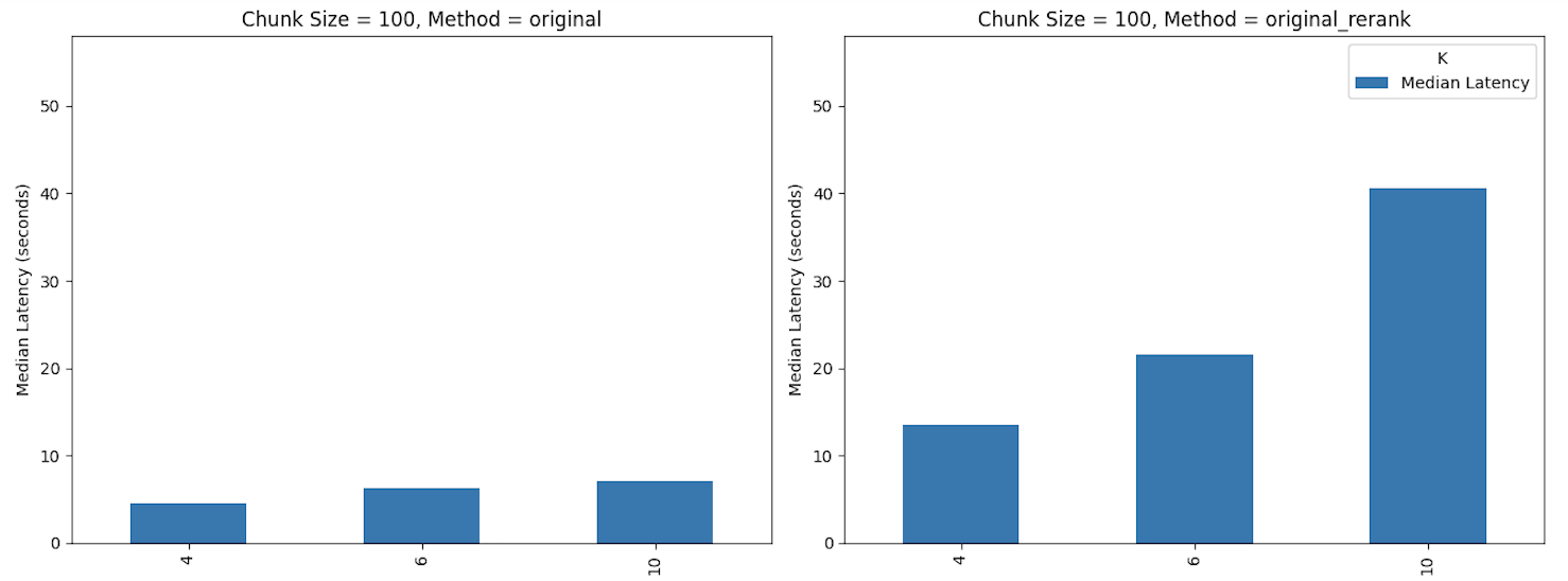
The above shows that as we increase K from 4 to 10, our latency almost doubles for the normal ranking method and skyrockets for re-ranking approaches. Most direct user experiences would lend themselves to the faster experience, say K=4, unless the performance metric makes a strong case for something else.

Chunking

Overview Basic Chunking Strategies

How you chunk data can be extremely important to the success of your search and retrieval efforts. Here are a few prevailing strategies for background.

1. Uniform chunking: Breaks down data into consistent sizes, often defined by a set number of tokens. 1 token is about 4 characters in English. While this strategy is straightforward, it risks dividing individual pieces of information across multiple chunks, which might lead to incomplete or incorrect responses.
2. Sentence-based chunking: Breaks down data on structural components like periods or new line characters. This strategy could do a better job of segmenting information, but again risks splitting information across multiple chunks. Some more advanced NLP libraries can help make divisions on these characters while preserving context.
3. Recursive chunking: Divides the text and then continuously divides the resulting chunks until they match defined size or structure conditions. While it can produce more contextually coherent chunks, the method is more resource-intensive than the others.

Choosing Chunk Size

Regardless of the strategy used to split chunks, choosing the size of the chunks can have a dramatic impact on the precision of system output. Smaller chunks might lead to only the most contextually relevant data coloring a chatbot’s output, but details that could have provided more context might be lost to adjacent chunks. Larger chunks might capture all relevant information to a query but could also contain irrelevant information, leading to less precise output.

What do the benchmark metrics tell us about chunk size?

The results of our evals on question-and-answer correctness show that sending too much information to the LLM’s context window causes issues. When chunk size becomes excessively large, such as exceeding 1000 tokens, we observe a decline in response accuracy.

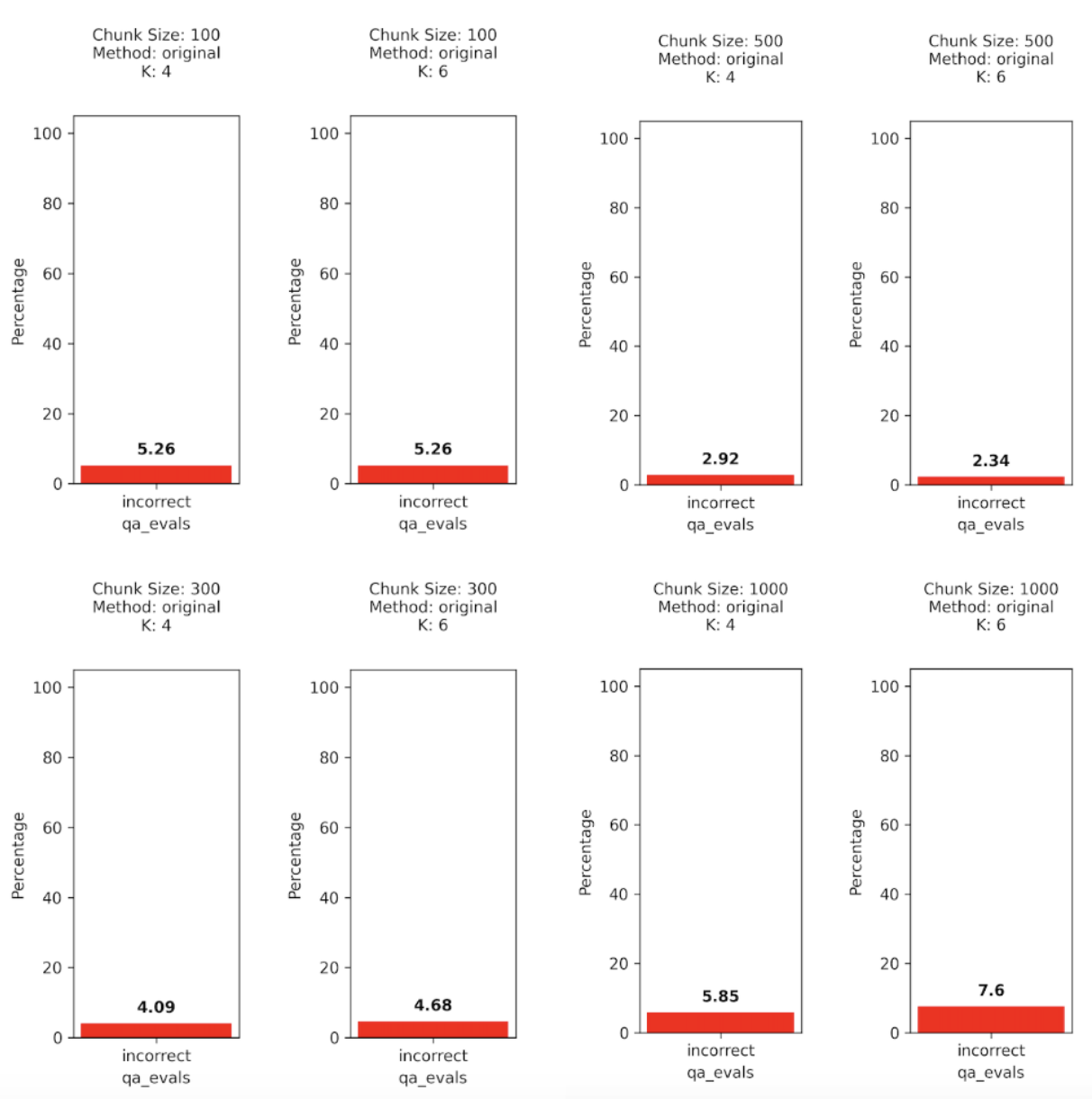
The graph above shows answer percent incorrect the larger the number the worse the results. There seems to be a sweet spot somewhere in between the smaller context of 100 tokens and the larger contexts of 1000 tokens.

Given the results so far we are leaning toward K = 4 and Chunk Size = 300/500.

Advanced Chunking Strategies

To navigate the aforementioned tradeoffs between large and small chunk sizes, different strategies have been developed to get the best of both worlds: the precise semantic meanings captured by small chunks and the overarching context of large chunks.

Langchain’s and LlamaIndex’s parent document retriever systems address this with a two-fold approach. Initially, the system matches user queries to relevant information in the vector store using precise, semantically-rich smaller chunks. Then, once the small chunks are identified, the system retrieves larger chunks that contain the identified smaller chunks as well as surrounding text. This strategy ensures that while the relevant information is pinpointed with accuracy, the delivered response is enriched by the broader context of the corresponding larger chunk.

Embedding

After chunking our data, the next step is to transform these text chunks into a format that the retrieval-based chatbot can understand and use (embedding).

Off-the-shelf embedding models exist for this, or training your own model might be the way to go. We find teams typically go with the embedding option available to them based on their companies’ data privacy needs and LLM vendor choice. If you use OpenAI, Ada-2 is great; if you have Google, Gecko is also a good option. In cases where you need an OSS embedding model, a number are available.

In the stage of just getting things working, simple embedding models can be fine. BERT embeddings are still used by many teams. As you look to really improve your results, the retrieval steps dictated by the embeddings, is the area that most teams can control the most.

Fine-tuning on embeddings is something teams are doing to improve their retrieval results. The OpenAI Ada-2 models currently don’t support fine tuning so the majority of use cases of improving embedding retrieval is based on OSS models or fine tuning done outside of OpenAI.

Again, there is no replacement for experimentation. Testing different models and configurations on your specific dataset is the best way to find your optimal solution.

Retrieval: Comparing Search Methods

After your data is chunked and embedded in your vector database, there are several techniques we can use to augment the retrieval process.

Multiple Retrievals and Reranking

Instead of retrieving only the most relevant chunk for your knowledge base, you can design your system to return a set number of the most relevant chunks in your database. Once you’ve retrieved this potentially relevant data, an LLM can rank the retrieved chunks based on its judgment of how relevant they are to the user’s query. Through this process, your system casts a wider net, returning multiple potentially relevant chunks before deciding which should be used to inform the ultimate output.

Self-Querying

When handed a question in natural language, a self-querying system uses an LLM to craft a more structured, standardized inquiry format - which it then runs against its vector store. This allows not only for semantic matching against saved documents but also for extracting and applying specific filters based on the nuances of the initial question.

Multiple Source Retrieval

Several RAG system frameworks already allow users to connect multiple databases to their system. In practice this could look like an internal system detailing your codebase having access to technical documentation, ticketing, relevant communications, or anything else necessary to handle user input.

Multi Query Retrieval

Document retrieval can be finicky, with results shifting based on minor changes in a query’s content. To mitigate this, the system expands on the user’s initial input, producing a range of related queries to capture different angles. Each variant then extracts its own batch of pertinent documents. These distinct batches are then pooled together, offering a comprehensive and consistent array of relevant documents.

Hypothetical Document Embeddings (HyDE)

This advanced strategy reframes retrieval as a two-step process: one part generative, one part comparative.

The generative stage begins with the query being inputted into a large language model. This model is then given a directive to “create a document that addresses the question.” This generated document doesn’t have to be real or even entirely factual. It’s a hypothetical representation of what an appropriate answer might look like.

Once the hypothetical document is constructed an embedding model translates this fictitious document into an embedding vector. It’s expected that the model would filter out any unnecessary details, acting as a compression tool that retains the crux while leaving out the fluff.

The vector is then matched against the established vector store to find the most fitting real-world, pre-existing documents. What’s interesting here is that HyDE doesn’t explicitly model or compute the similarity score between the query and the returned document. The process instead focuses on natural language understanding and generation tasks, with retrieval effectively transformed into these two components.

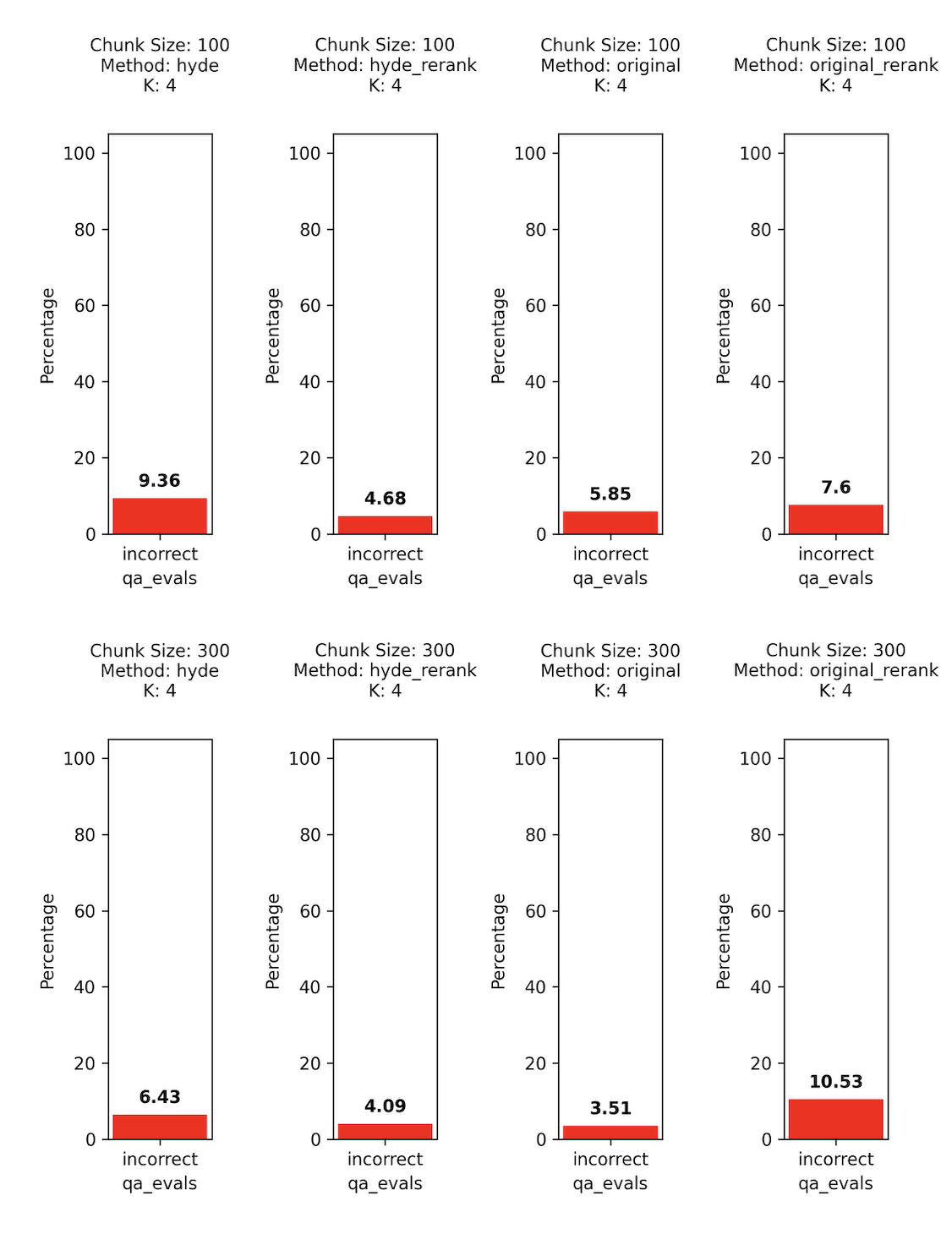
In looking at the above example, the HyDE with re-rank does outperform most of the other options, but it is very slow. The re-rank alone’s poor performance surprised us. What we found is that sometimes the re-rank by itself will cause the best quality chunk to go from #1 to #2-#4, and that small movement might be the cause for some missed answers.

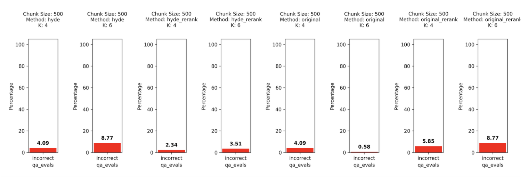
Again, here the HyDE + re-rank does outperform on most of the options but the delay is quite large. The increase in K in almost all cases, makes the answers worse.

There is a lot to dig into but at a quick glance a simple retrieval with a small K=4, chunk size 300–500 and original embedding retrieval looks like a good fit for fast responses. If you have time to wait, the HyDE + re-rank could be an option as well.

Conclusion

Conclusion
Check out the test scripts and notebook for an example on how to parameterize retrieval on your own docs, leverage LLM evaluations, and reproduce results.
Ultimately, experimenting with different options in the setup of your RAG system will lead to the best outcome with your specific use case and data. There are many different chunking methods, chunk sizes, embedding models, retrieval techniques and more to try out, and the only way to find which is to test.