Data Binning Challenges in Production: How To Bin To Win

Learn how to handle common challenges with feature binning for your model’s use case to optimize monitoring, alerting, and root cause analysis in production.

What Does It Mean To Bin Data?

Binning, also known as bucketing or discretization, is a data processing technique for reducing the cardinality of continuous and discrete data. Whether used in data pre-processing or post-processing, binning divides data from numeric features into a set of discrete intervals assigning each data point to its corresponding bin.

For example, let’s say you have a machine learning (ML) model that predicts housing prices and the numeric feature for square footage ranges from 1000 to 25000 square feet. To bin this data you could create equal width bins or bins with a similar number of values assigned to each bin. For equal width bins let’s say you divide the data into 25, 1000 unit bins – now you can simplify your data analysis and set monitors in production. However, in order to calculate model drift, you need to make sure the bins in your training and production distributions meet certain criteria. Let’s say after a month, your model in production starts to decay because it is underpricing houses outside of square footage ranges from 1000 to 25000. How can you learn that your model is doing this before the house actually sells at the poorly predicted price? In this piece, you will see that detecting model insights, calculating drift, root causing and resolving issues in production, all start with binning.

Why Does Binning Data Become Complicated?

When discussing the subject of ML observability, the biggest complications with monitoring and troubleshooting models in production are usually around the data – data integrations, data drift, data quality checks and inference data pipelines. While these data hurdles are imperative to address to keep models performing optimally in production, a complicated topic that often goes overlooked is binning strategy.

The binning of data seems like a straightforward task until you come across sparse and low volume data, it is at this point where we see that binning is much more complex than it appears. The normal challenges of binning are exacerbated in production by a number of factors, including the need for automated binning approaches and the fact that most ML teams are continuously adding new data (that ultimately changes data distributions). The more teams have to manually configure a binning strategy to understand their model behavior, the more likely they are to miss key model insights. This has a cascading impact and can lead to a misrepresentation of the model, which can be responsible for customer churn, user dissatisfaction, and loss in profitability for a company.

In this piece, we discuss:

• The role binning plays in monitoring your models in production.
• Why binning is a challenge when setting up feature drift monitors.
• The binning strategies you need to be aware of when setting up monitors for your model use case.
• How to start using these new binning techniques to monitor your models in production today.

The Role of Binning In Drift

To understand the role of binning, we first need to talk about drift. In machine learning systems, drift monitoring is critical to delivering quality ML.

When To Use Drift Metrics

Drift is used as a proxy for model performance when teams are unable to receive a ground truth in a timely manner. Whether their ML models receive delayed actuals (churn models) or few actuals (customer lifetime value models), drift analysis use cases in production ML systems include:

• Detect feature changes between training and production to catch problems ahead of performance degradation
• Detect prediction distribution shifts between two production periods as a proxy for performance changes (especially useful in delayed ground truth scenarios)
• Use drift as a signal for when to retrain – and how often to retrain
• Catch feature transformation issues or pipeline breaks
• Detect default fallback values used erroneously
• Find new data to go label
• Find clusters of new data that are problematic for the model in unstructured data
• Find anomalous clusters of data that are not in the training set
• Find drift in embeddings representing image, language, or unstructured data

The problems above have plagued teams for many years, and while there is no perfect metric to solve every drift challenge in production, we have written detailed pieces in an attempt to bring more clarity to these drift metrics and how they are used in model monitoring. Some of the most popular metrics for monitoring drift include, population stability index (PSI), Kullback-Leibler (KL) divergence, Jensen Shannon (JS) divergence, and the Kolmogorov Smirnov (KS) test. In model monitoring, we almost exclusively use the discrete form of PSI and KL to obtain the discrete distributions by binning data. The discrete form and continuous forms of these metrics converge as the number of samples and bins approach infinity.

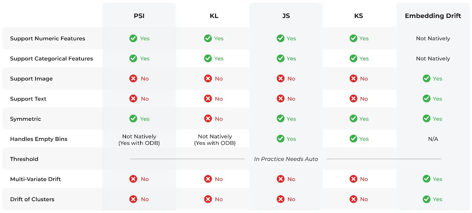
The above table gives a good breakdown of some of the most commonly-used drift metrics and statistical distance checks.

The Challenges of Binning

In production, ML teams are almost exclusively working with binned distributions for structured data. Interestingly, how one creates bins can impact drift monitoring more drastically than the metric selection itself. As seen from the table above, not all drift metrics “Handle Empty Bins.” With KL Divergence and PSI, if you don’t modify the equations for binning then comparing 0 bins will cause the values to go to infinity. This is due to the zero in the denominator causing a divide-by-zero, the nature of KL divergence, and ultimately how these distributions behave. KL and PSI can’t mathematically handle zero bins because these distributions are the solution to an optimization problem which breaks down in the presence of those zeros.

Since KL divergence becomes infinite and the gradient signal becomes zero, JS divergence may be seen as better behaved in the sense that it doesn’t become infinite with zero bins, but it suffers from the same problem of having zero gradient when there is little or no overlap. JS is essentially the symmetric and smoothed version of the KL divergence. Now, you may be wondering why it is often a better option to add a modification to PSI than to use JS in production. Long story short,  JS divergence is calculated by creating a mixture distribution that changes every time you run a comparison because the production distribution changes every sample period. This is not ideal for consistent drift monitoring. See “Population Stability Index (PSI): What You Need To Know” and “Jensen Shannon Divergence: Intuition and Practical Application” to understand the full picture.

Strategies and Solutions

In the pieces from our machine learning course, we discussed why PSI is one of the most stable and useful metrics for monitoring drift at scale and in production. Now we need to decide how to use PSI to monitor ML models with difficult binning cases.

Solution 1: Modify the Data

You can throw out all the values that do not make sense. For KL Divergence, for example, this means ignoring divide by zero and infinity errors by either erasing them or setting them as zero.

Solution 2: Smooth the Distribution 

You can use smoothing by taking a Bayesian prior or Dirichlet prior, which amounts to treating each entry as a fraction. This may be problematic for interpretation and is unlikely to remain stable and scalable down the line.

Another heuristic solution we see often is called Laplace smoothing that adds 1 to all zero bins (it just slightly changes the distribution).

The problem with the approach is that it assigns an almost zero probability to the event occurring. If it does occur (distribution A has counts much higher than 1) it can cause spikes in KL divergence based on your choice of Laplace Smoothing.

Solution 3: Modify the Algorithm

At Arize, we have a unique algorithm to handle zero bins called out-of-distribution binning (ODB) that we will outline in a future blog.

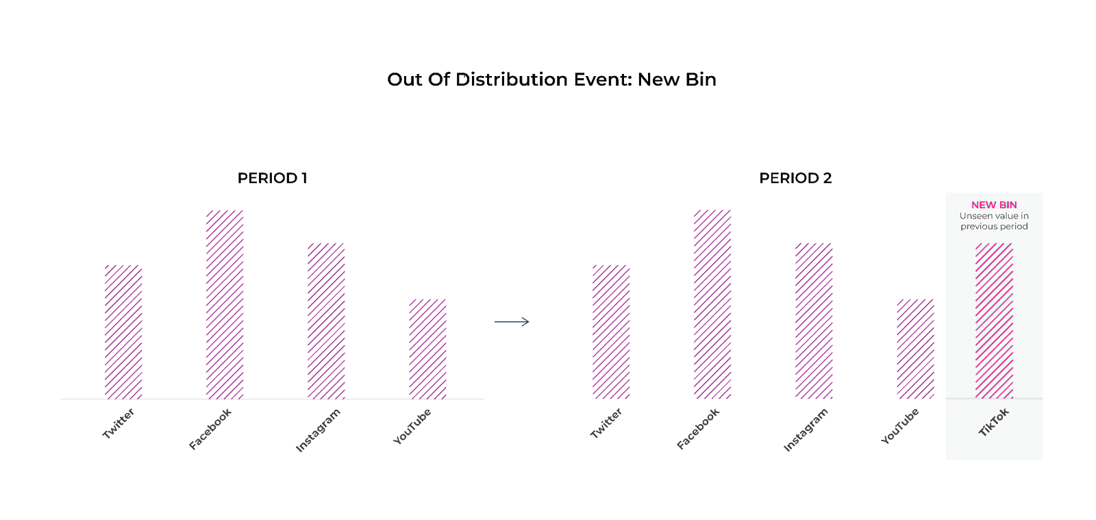
Terminology

• Equal width/bin size: This method involves dividing the range of the variable into equal intervals of the same width.
• Equal frequency/bin count: This method involves dividing the data into bins with an equal number of data points in each bin.
• Manual/binning: Manually define bins based on expert knowledge or specific requirements of the analysis.
• Quantiles: Ways of dividing a dataset into smaller groups based on a certain percentage or proportion of the data.
  • Percentile: A measure that indicates the percentage of data that falls below a certain value. For example, the 99th percentile is the value below which 99% of the data falls.
  • Decile: A way of dividing a dataset into 10 equal parts, with each part containing 10% of the data.
  • Quintile: A way of dividing a dataset into five equal parts, with each part containing 20% of the data. The first quintile represents the 20th percentile, and the fourth quintile represents the 80th percentile.
  • Quartile: A way of dividing a dataset into four equal parts, with each part containing 25% of the data. The first quartile represents the 25th percentile, the second quartile represents the 50th percentile (or the median), and the third quartile represents the 75th percentile. Commonly used for a box and whisker plot (see below for an example).
  • Median: The value that separates a dataset into two equal parts, with 50% of the data above and 50% below. It is also known as the 50th percentile.

Categorical vs. Numeric

Categorical Feature Binning

Distribution comparisons are useful for both visualizing data and calculating drift metrics such as PSI.

For categorical values, we simply calculate the percentage of data that falls under each unique value and display the data in descending order of data volume.

For numeric features, it often makes sense to group the values into bins in order to show a useful summary of the data. However, there is no one-size-fits-all strategy for numeric binning that will work for a wide variety of data shapes. We cover the best option for each use case below.

✏️ NOTE: In the case of categorical features, when the cardinality gets too large the measure starts to lose meaning.

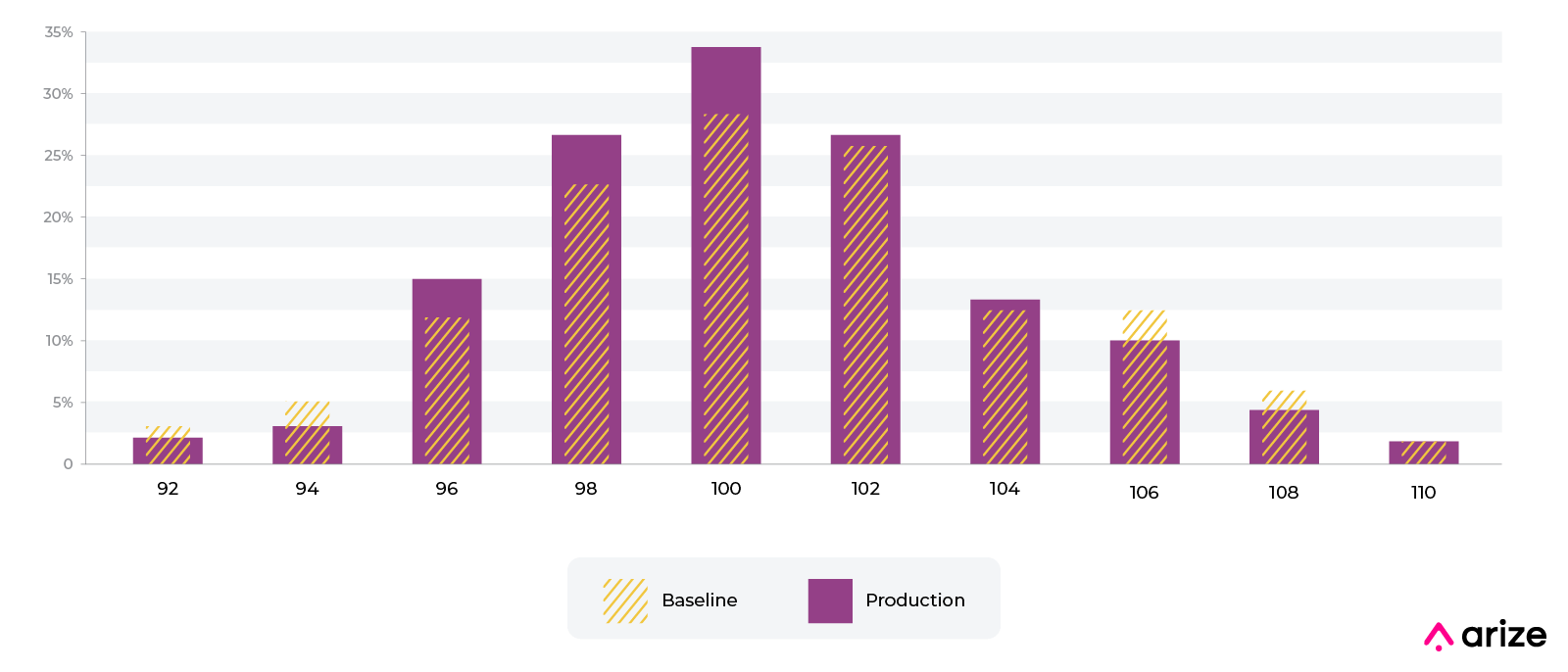
Numeric Feature Binning

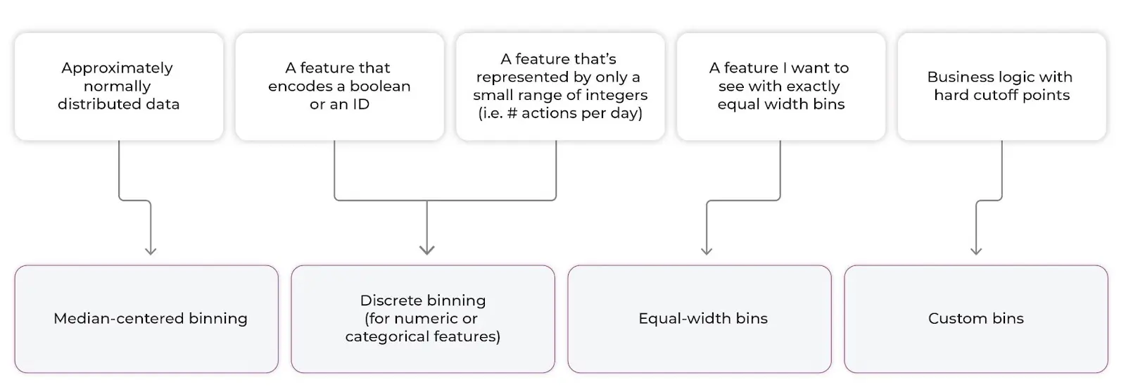
We recommend four types of binning strategies for numeric features:

1. Median-centered binning
2. Discrete binning (For numeric or categorical features)
3. Equal width bins
4. Custom bins

Quick guide:

Median-Centered Binning

Understanding Quartiles and Quintiles for Numeric Bins

Quantile Binning:
Quantiles are most commonly associated with box plots, which are helpful to visualize your data. In the case of quantile binning for histograms, the edges of the bins are determined by quantile cuts.

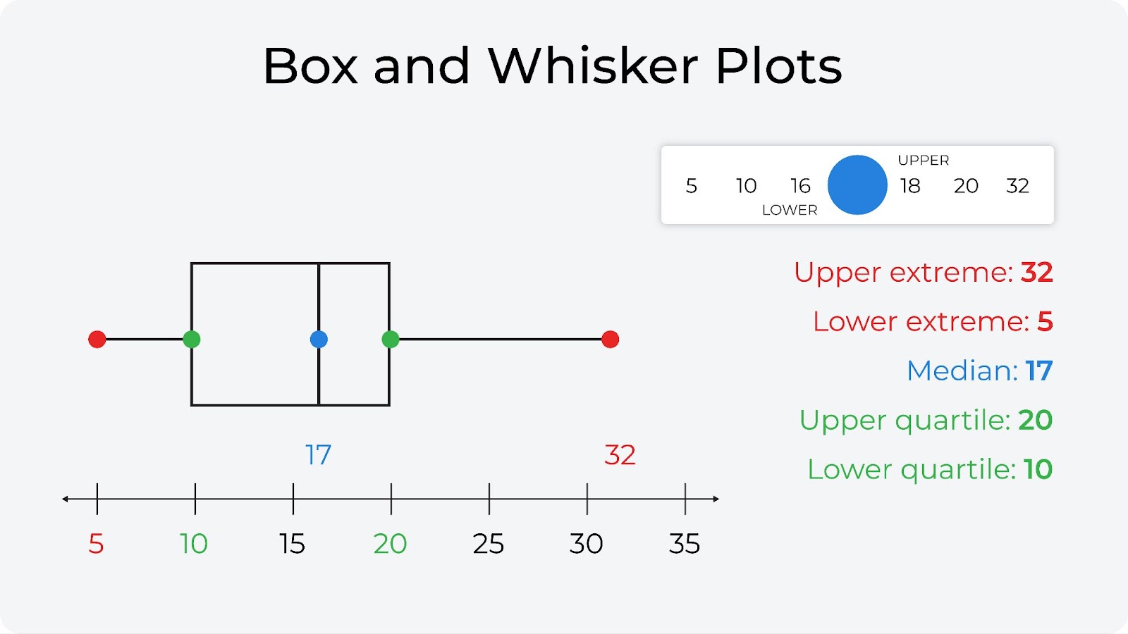
In a lot of ad-hoc analysis quantile binning can be quite helpful, but as a view for quick production analysis it is often problematic in our experience. First, in production, you are always comparing two distributions and it is not so clear where all the bin cuts should be to drive helpful insights. The other challenge is that the bin widths are not necessarily uniform and can be hard to visualize in a lot of cases.

Even Binning with Quantile Edges, also known as Median-Centered Binning

At Arize, this is our most common binning approach. It takes a bit of the best features from quantile binning and even binning. The outliers are handled by edge bins that include the infinity bins; they act like quantile edge bins typically at 10% and 90% cuts. Everything in between 10% and 90% points are evenly binned so there is even bin width in the middle. We did not create this binning approach – it’s used in finance quite often, for example – but find that most users really like the advantages.

Median-centered binning works well for normally distributed data but is good for highly skewed data as well.

This method creates up to 10 bins, with the following constraints:

1. The center of the bins (the division between bins 5 and 6) is at the median.
2. The 8 center bins have equal width. The width of each bin is ⅓ of the standard deviation of the data. These are the purple squares below.
3. The edge bins have variable width and end at the min/max of the dataset in order to account for long tails. These are the red rectangles below.
4. Bins on the edge with 0% of the data will be removed – possibly producing less than 10 bins.

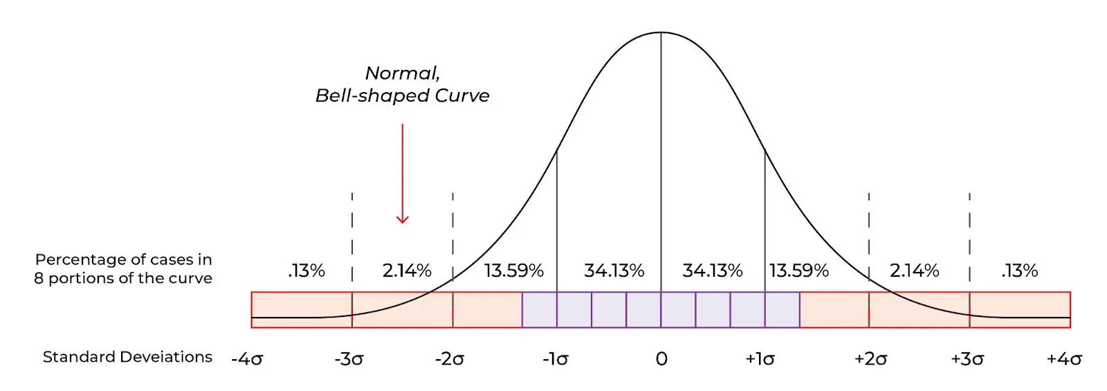
This works very well for most normally distributed data, even if there is a long tail. For example, take the annual income feature in our model below. Income is normally distributed within a range, with a long tail on the right for high earners. In Arize, this feature is binned like this:

The majority of the data is centered around media income of $43,000, while about 30% of the data falls into the left and right edge bins.

Discrete Binning

Discrete binning allows users to see each value independently in the distribution chart. Note that for categorical features, this is the only binning option.

For numeric features, this works particularly well for these use cases:

Booleans or IDs

Sometimes, a boolean value or an ID may be expressed as an integer. Since the numeric value of these features is not actually relevant, using median-centered binning above would not produce the right results. For example, below is what a boolean value looks like with median-centered binning. Since the bin has 100% of the dataset, it is impossible to calculate a meaningful drift value using PSI or other drift metrics.

By choosing discrete binning, you can easily see the distribution of the only two values for this feature, 0 and 1:

In this example, we have an ID for a type of procedure, encoded as an integer. Median-centered binning combines multiple values because they are numerically close. However, for IDs this doesn’t make sense as the values have no numeric meaning.

By choosing discrete bins, users can see the frequency of each ID independently.

Small Integer Values

For small integer ranges, such as a count, discrete binning offers a more detailed view of the data than median-centered binning.

For example, this is a count of the orders in a day. With a small number of unique values, discrete binning offers a more granular view of the data.

Equal Width Bins

Also known as even binning, this approach is intuitive and the most straightforward of the approaches to implement.

Even binning is implemented by taking the edges of the distribution and then evenly breaking up the distribution into N bins. Each bin is the same width and visually it is easy to understand.

The problem with even binning is outliers. The more the distribution has extreme ends or concentrations of data, the more skewed even binning can appear. This can manifest in viewing the data with a single bin. In practice, we find a high percentage of distributions are problematic to visualize with even binning.

This option can be useful for fixed numeric ranges like FICO scores, for example.

Custom Bins

Custom bins offer ultimate control over the visualization of numeric data. This is helpful when you already know how to visualize your data, either from prior analysis, or from a business perspective where certain cutoffs already exist.

Using the same FICO score example, creditors may have certain cutoffs for FICO scores. Say, a FICO score below 500 results in an automatic application rejection. For scores above 500, every 20 points results in a better interest rate than the previous bucket.

Aligning the binning strategy with business logic ensures the drift visualization is relevant.

Takeaways

When designing a winning binning strategy, it’s important to consider the nature of the data and the drift metric criteria. If monitoring models in production is a new endeavor for your team, you should experiment with several binning techniques to see which method best fits the data. The choice of bin size and binning technique can impact the effectiveness of your feature drift monitors in production. In Arize, you can test out a variety of drift evaluation metrics, customized to monitor for all types of datasets at scale in production. Ultimately, the methods shown here improve our drift calculations and speed up root cause analysis data issues to best serve your ML models in production.