Jensen Shannon Divergence: Intuition and Practical Application

What Is JS Divergence (JS Div)?

The Jensen-Shannon divergence (JS) metric – also known as information radius (IRad) or total divergence to the average – is a statistical measurement with a basis in information theory that is closely related to Kullback-Leibler divergence (KL Divergence) and population stability index (PSI). The advantage of JS divergence over other metrics is mostly related to issues with empty probabilities for certain events or bins and how these cause issues with KL divergence and PSI. The JS divergence metric uses a mixture probability as a baseline when comparing two distributions as its main contribution. In the discrete versions of PSI and KL divergence, the equations blow up when there are 0 probability events.

This post covers:

• What is JS Divergence and how is it different from KL Divergence
• How to use JS Divergence in machine learning model measurement
• How the unique approach of a mixture distribution helps with a common measurement issue
• Problems with a mixture distribution in model measurement

Jensen-Shannon Divergence (JS Divergence) Overview

Jensen-Shannon is an asymmetric metric that measures the relative entropy or difference in information represented by two distributions. Closely related to KL Divergence, it can be thought of as measuring the distance between two data distributions showing how different the two distributions are from each other.

The following shows the symmetry with KL Divergence:

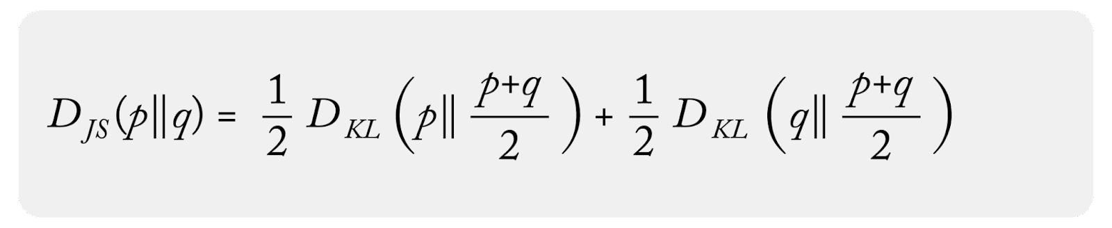
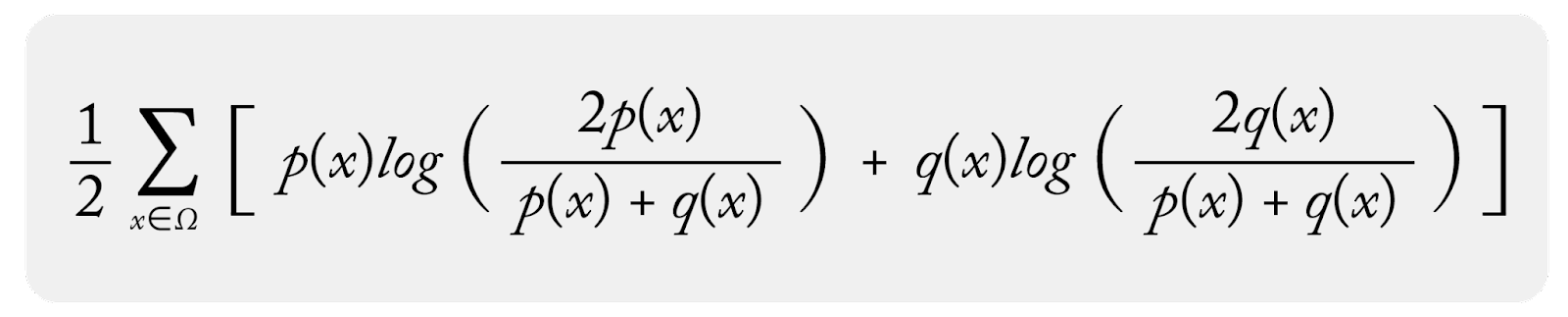
And here is a discrete form of JS Divergence:

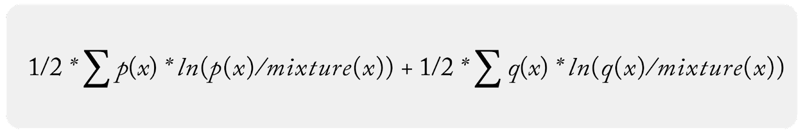
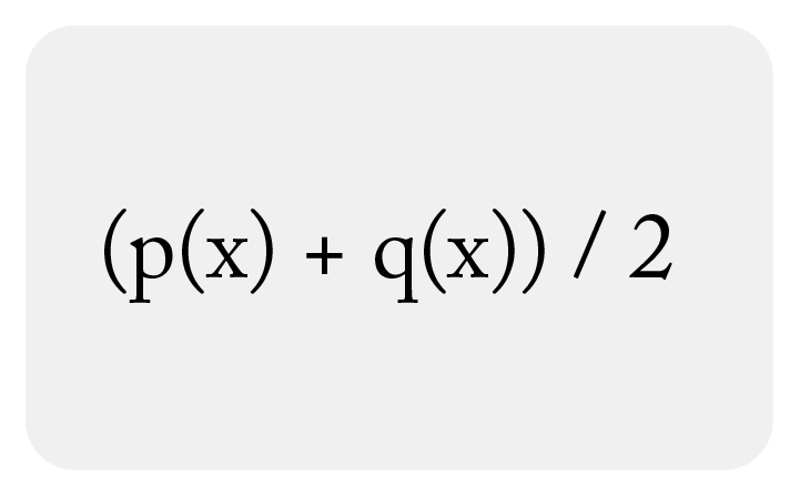
Where the mixture distribution is:

Frank Nielsen of Sony Computer Science Laboratories authored one of the better technical papers on JS Divergence.

In model monitoring, we almost exclusively use the discrete form of JS divergence and obtain the discrete distributions by binning data. The discrete form of JS and continuous forms converge as the number of samples and bins move to infinity. There are optimal selection approaches to the number of bins to approach the continuous form.

How Is JS Divergence Used In Model Monitoring?

In model monitoring, JS divergence is similar to PSI in that it is used to monitor production environments, specifically around feature and prediction data. JS divergence is also utilized to ensure that input or output data in production doesn’t drastically change from a baseline. The baseline can be a training production window of data or a training/validation dataset.

Drift monitoring can be especially useful for teams that receive delayed ground truth to compare against production model decisions. Teams rely on changes in prediction and feature distributions as a proxy for performance changes.

JS divergence is typically applied to each feature independently; it is not designed as a covariant feature measurement but rather a metric that shows how each feature has diverged independently from the baseline values. Although JS divergence does uniquely support a multi-distribution mixture approach, it really is not designed for comparing completely disparate distributions — it’s not a mulit-variate drift measurement.

The challenge with JS divergence – and also its advantage – is that the comparison baseline is a mixture distribution. Think of JS Divergence as occurring in two steps:

Step 1:

Create mixture distribution for comparison using the production and baseline distributions;

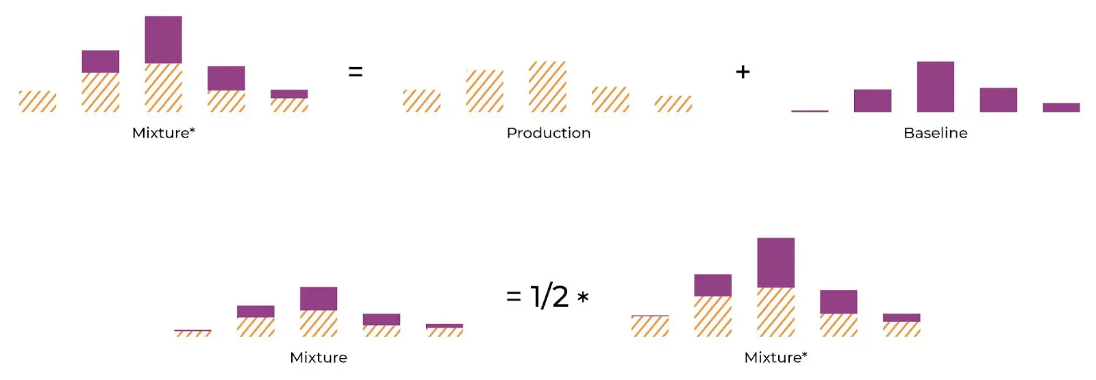
Step 2:

Compare production and baseline to mixture.

The above diagram shows the A distribution, B distribution and mixture distribution. The JS Divergence is calculated by comparing the JS distribution to both A & B.

✏️NOTE: sometimes non-practitioners have a somewhat overzealous goal of perfecting the mathematics of catching data changes. In practice, it’s important to keep in mind that real data changes all the time in production and many models extend well to this modified data. The goal of using drift metrics is to have a solid, stable and strongly useful metric that enables troubleshooting.

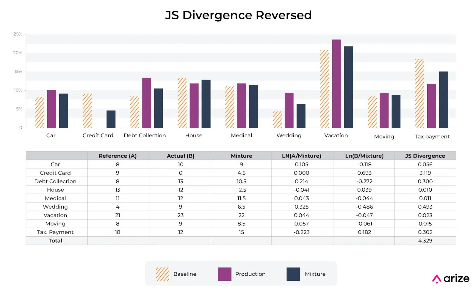
JS Divergence Is a Symmetric Metric

JS divergence is similar to PSI in that it is a symmetric metric. If you swap the baseline distribution p(x) and sample distribution q(x), you will get the same number. This has several  advantages compared to KL divergence for troubleshooting data model comparisons. There are times where teams want to swap out a comparison baseline for a different distribution in a troubleshooting workflow, and having a metric where A / B is the same as B / A can make comparing results much easier.

This is a reason Arize’s model monitoring platform defaults to population stability index (PSI), a symmetric derivation of KL Divergence, as one of the main metrics to use for model monitoring of distributions.

JS Divergence Advantage: Handling Zero Bins

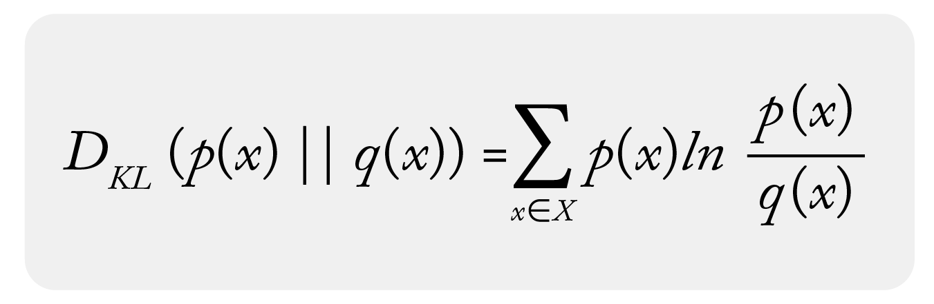
The main advantage of JS divergence is that the mixture distribution allows the calculation to handle bin comparisons to 0. With KL Divergence, if you are comparing 0 bins the equation essentially blows up.

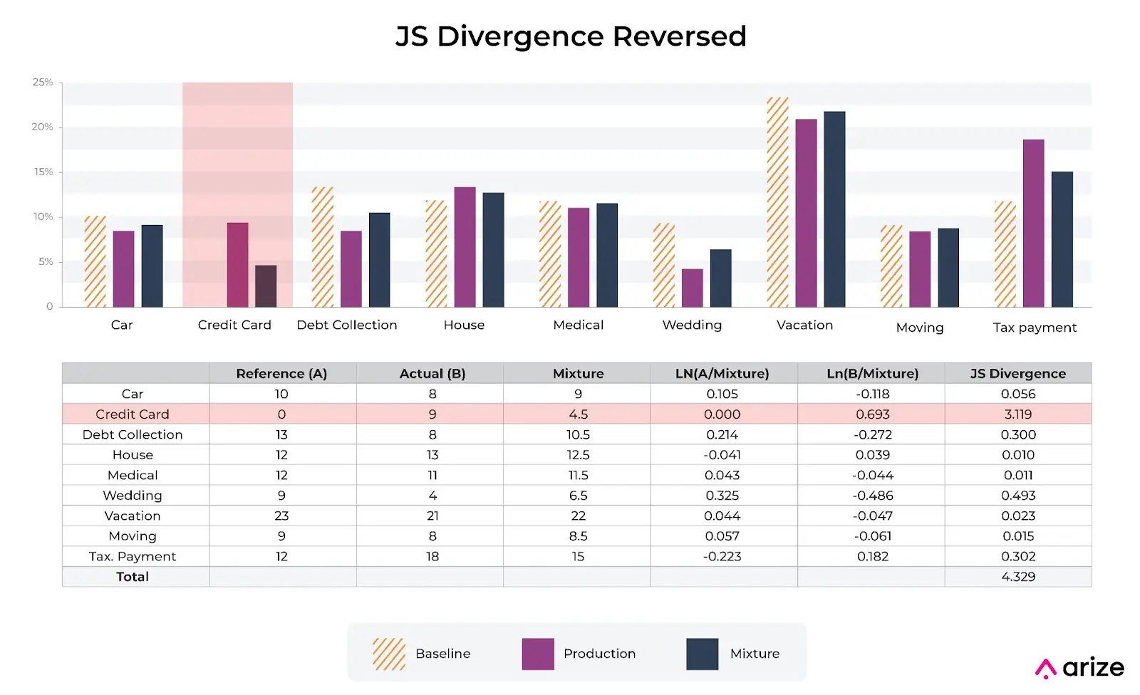
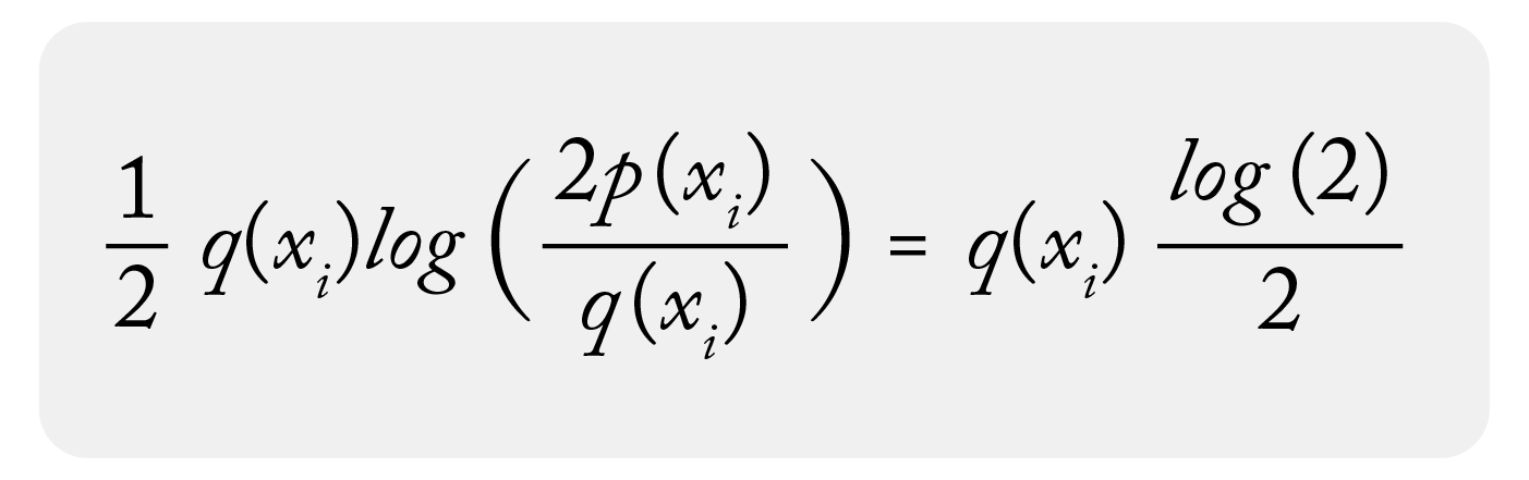
As you can see in the image above, there are two buckets where one bucket is 0 in the current time frame and the other has a value. The approach with JS Divergence to handle the 0 bucket is to take the two terms in JS Divergence and assume one is 0 (0*ln(0) = 0) as the function is smooth and has a limit as it approaches 0 and the other has a value:

Assuming one term is 0, you have for the 0 bin:

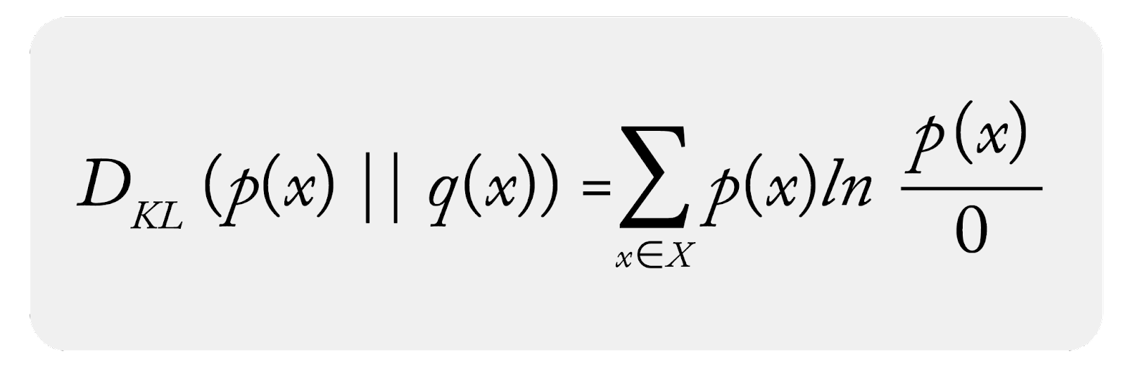
This will not work with KL divergence or PSI as you would divide by 0 in the denominator:

In the case where q(x) = 0 you have:

Advantage: The zero bins are handled naturally without issue

✏️NOTE: Arize uses a unique modification (to be outlined in a future writeup on binning) that allows KL Divergence and PSI to be used on distributions with 0 bins. The modification is designed specifically for monitoring and might not be applicable to other use cases.

JS Divergence Disadvantage: Mixture Distribution Moves

The disadvantage of JS divergence actually derives from its advantage, namely that the comparison distribution is a “mixture” of both distributions.

In the case of PSI or KL divergence, the baseline comparison distribution is static comparison distribution, fixed in every comparison time period. This allows you to get a stable metric that means the same thing on every comparison and in every period. For example, if you have a PSI value on one day of 0.2 then a week later it is 0.2 this implies the entropy difference to the baseline is the same on both of these days. That is not necessarily the case with JS divergence.

In the case of JS divergence, the mixture distribution changes every time you run a comparison because the production distribution changes every sample period.

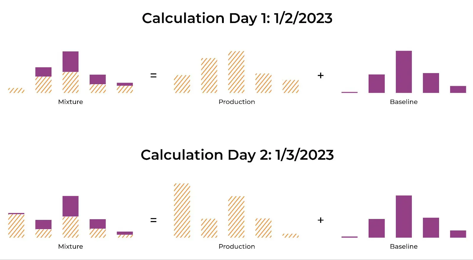
Calculation of Mixture Distribution for Each Monitoring Day

The chart above shows an example of a mixture distribution calculated for two different timeframes. The mixture acts like a slowly moving baseline that smoothly connects the baseline at time A with time B by averaging differences.

Differences Between Continuous Numeric and Categorical Features

JS divergence can be used to measure differences between numeric distributions and categorical distributions.

Numerics

In the case of numeric distributions, the data is split into bins based on cutoff points, bin sizes and bin widths. The binning strategies can be even bins, quintiles and complex mixes of strategies that ultimately affect JS divergence (stay tuned for a future write-up on binning strategy).

Categorical

The monitoring of JS divergence tracks large distributional shifts in the categorical datasets. In the case of categorical features, often there is a size where the cardinality gets too large for the measure to have much usefulness. The ideal size is around 50-100 unique values – as a distribution has higher cardinality, the question of how different the two distributions and whether it matters gets muddied.

High Cardinality

In the case of high cardinality feature monitoring, out-of-the-box statistical distances do not generally work well – instead, it is advisable to use one of these options instead:

1. Embeddings: In some high cardinality situations, the values being used – such as User ID or Content ID – are already used to create embeddings internally. Arize embedding monitoring can help.
2. Pure High Cardinality Categorical: In other cases, where the model has encoded the inputs to a large space, just monitoring the top 50-100 top items with JS divergence and all other values as “other” can be useful.

Of course, sometimes what you want to monitor is something very specific – like the percent of new values or bins in a period. These are better set up with data quality monitors.

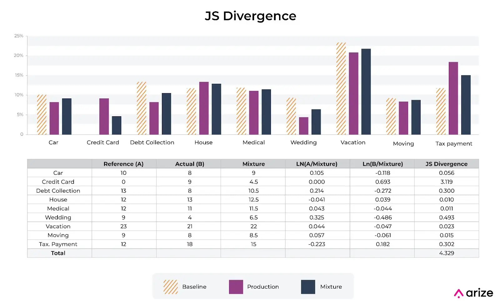
JS Divergence Example

Here is an example of JS divergence with both numeric and categorical features.

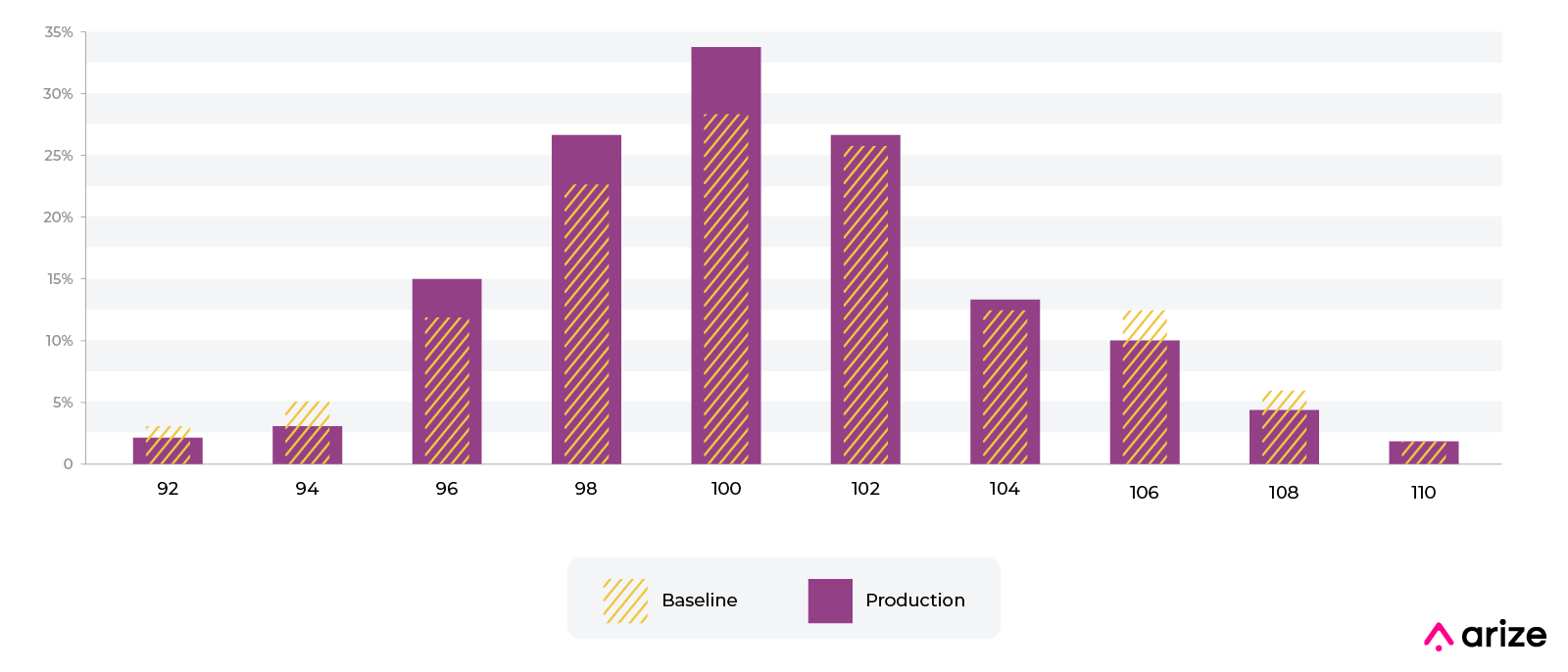
Imagine you work at a credit card company and have a numeric distribution of charge amounts for a fraud model. The model was built with the baseline shown in the picture above from training. We can see that the distribution of charges has shifted. There are a number of industry standards around thresholds for PSI but as one can see the values are very different for JS divergence. The 0.2 standard for PSI does not apply to JS divergence. At Arize, we typically look at a moving window of values over a multi-day period to set a threshold for each feature.

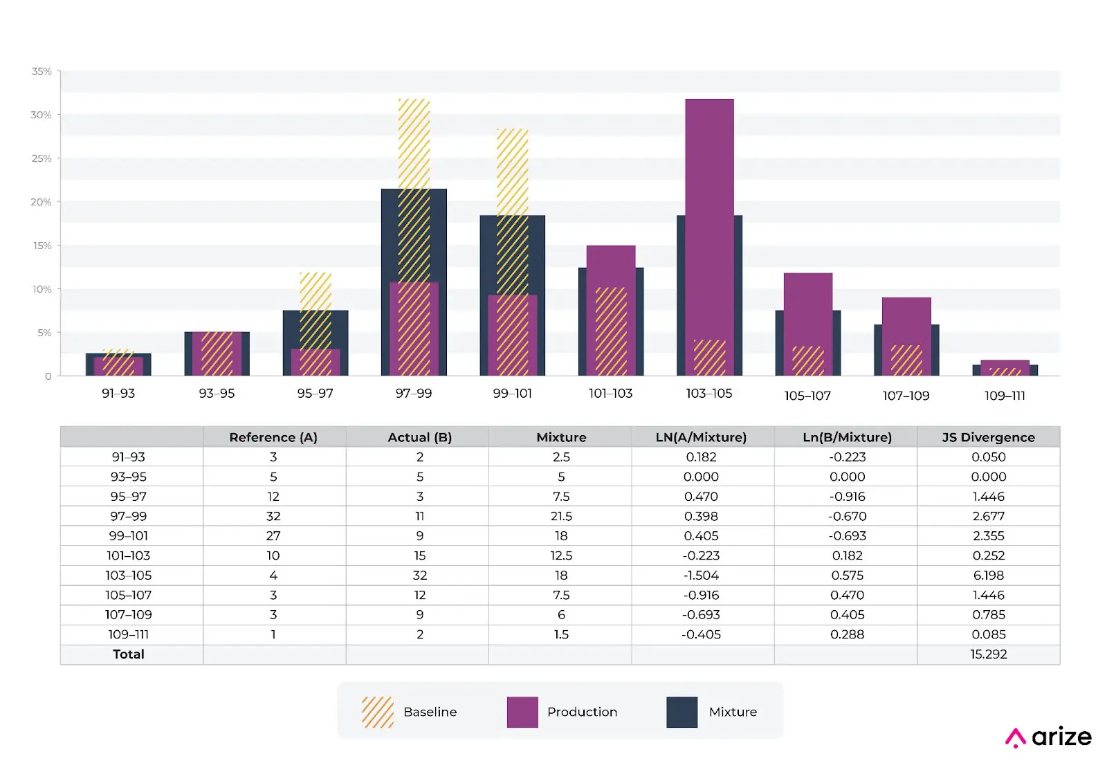
The example shows a numeric variable and JS divergence over the distribution. In the example above, it’s worth noting that a nine point drop from 12% to 3% for bin 95-97 causes a 1.4 movement in JS. This is exactly mirrored by a nine point increase from 3% to 12% for bin 105-107. PSI works in a similar symmetric manner to JS. This is not the same for KL divergence. In the case of KL Divergence, the 12%->3% causes a larger movement in the number.

Intuition Behind JS Divergence

It’s important to intrinsically understand some of the logic around the metric and changes in the metric based on distribution changes.

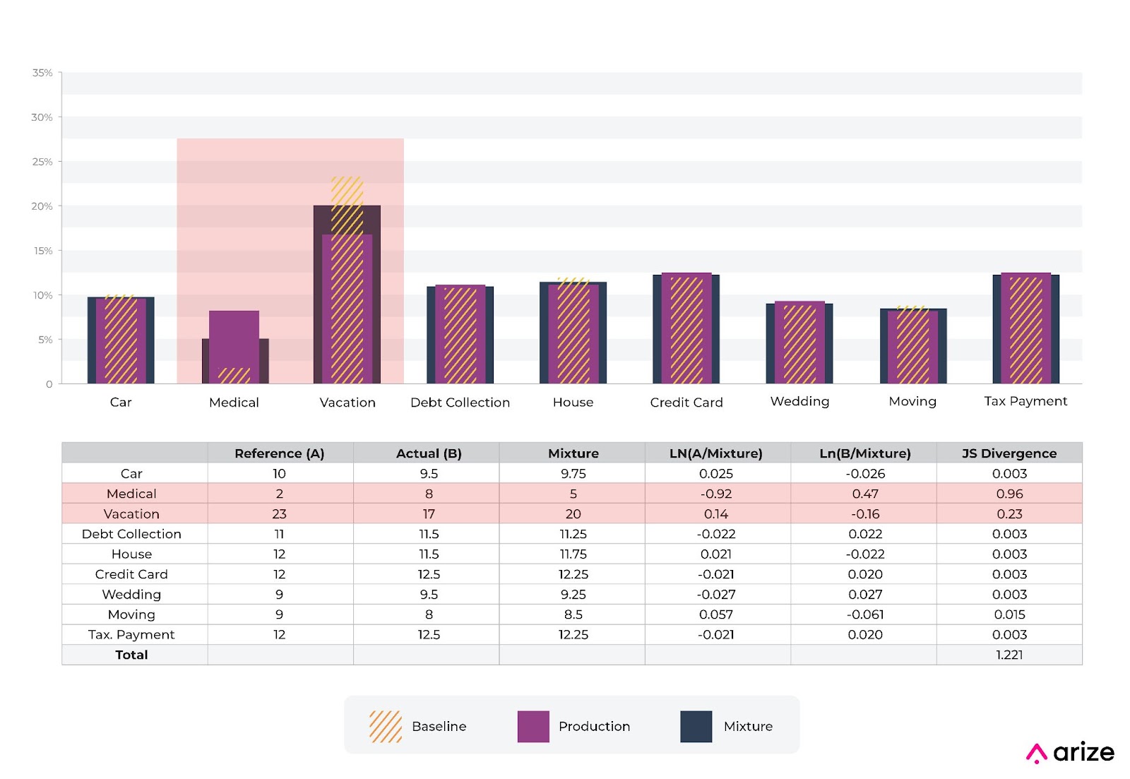
The above example shows a move from one categorical bin to another. The predictions with “medical” as input on a feature (use of loan proceeds) increase from 2% to 8%, while the predictions with “vacation” decrease from 23% to 17%.

In this example, the component to JS divergence related to “medical” is 0.96 and is larger than the component for the “vacation” percentage movement of 0.023. This is the opposite of what you get with KL divergence.

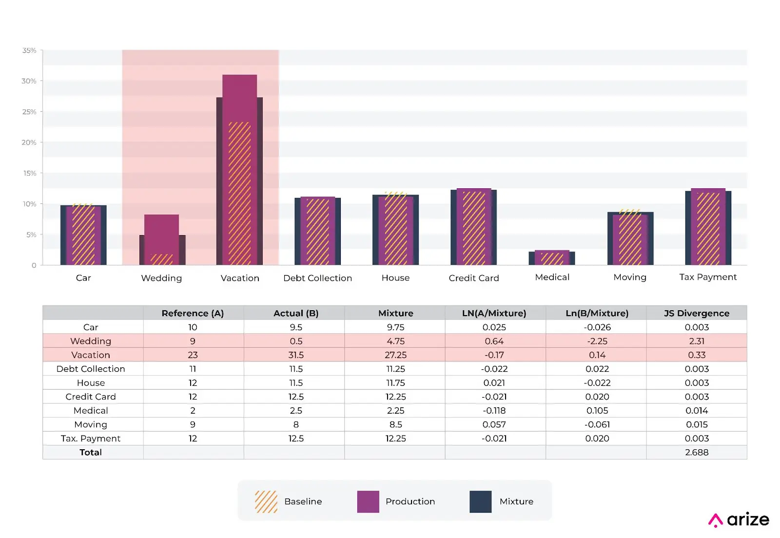
The example used in a previous post about PSI – which shows a large movement needed to get to a 0.2, a very basic but much used threshold – moves JS by a lot here. In this example, moving a bin from 9% to 0.5% moves JS by 2.31.

Here is a spreadsheet for those that want to play with and modify these percentages to better understand the intuition.

Conclusion

JS divergence is a common way to measure drift. It has some great properties in that it is symmetric and handels the 0 bin comparison naturally but also has some drawbacks in the moving mixture as a baseline. Depending on your use case, it can be a decent choice for a drift metric.

That said, Arize’s recommendation is for teams to use PSI along with an out-of-distribution binning technique to handle zero bins naturally. The out-of-distribution binning technique allows teams to both dial in how sensitive you want the metric to be out of distribution events and easily compare to a fixed baseline distribution (there is no mixture) – a best of both worlds scenario that has been tested and proven by the Arize team across tens of thousands of model monitors.

Stay tuned for additional pieces covering binning best practices and other recommended drift metrics.