


ARIZE MACHINE LEARNING COURSE
 The Fundamentals
The Value of Performance Tracing In Machine Learning

Key Components of Observability
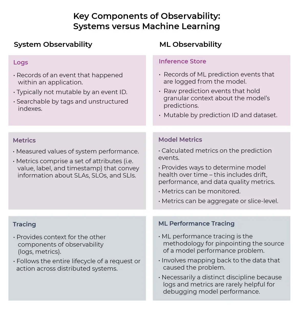
In infrastructure and systems, logs, metrics, and tracing are all key to achieving observability. These components are also critical to achieving ML observability, which is the practice of obtaining a deep understanding into your model’s data and performance across its lifecycle.
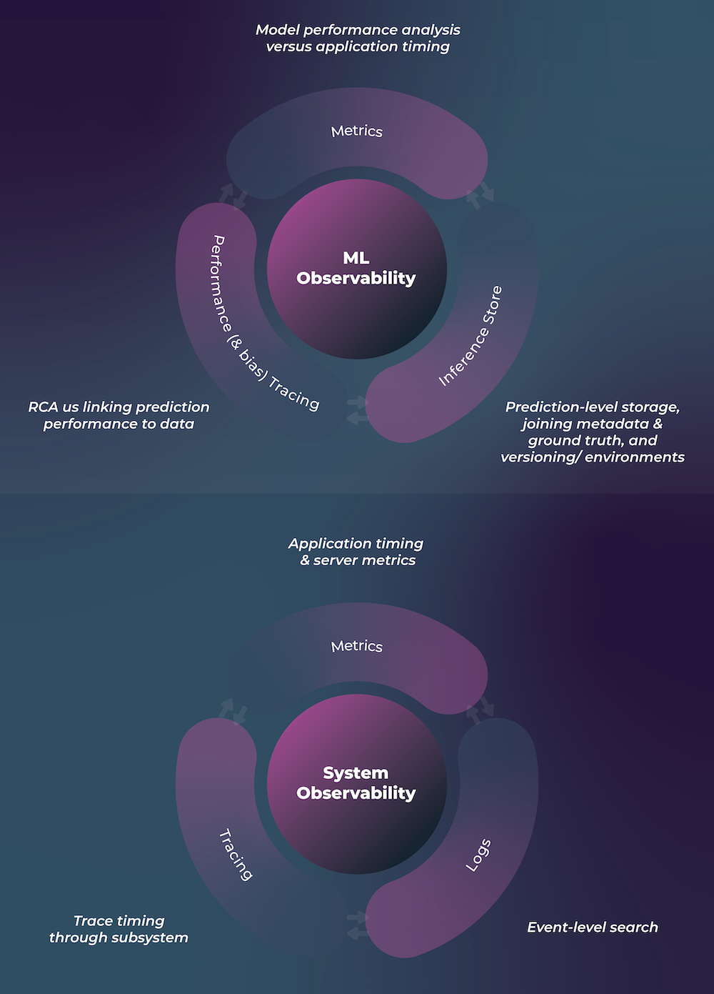
Inference Store – Records of ML prediction events that were logged from the model. These are the raw prediction events that hold granular information about the model’s predictions. There are some key differences between what logs in system observability means and an inference store in ML Observability. Will cover this in an upcoming post!
Model Metrics – Calculated metrics on the prediction events to determine overall model health over time – this includes drift, performance, and data quality metrics. These metrics can then be monitored.
ML Performance Tracing – While logs and metrics might be adequate for understanding individual events or aggregate metrics, they rarely provide helpful information when debugging model performance. To troubleshoot model performance, you need another observability technique called ML performance tracing.
In this piece, we will dive into how to use ML Performance tracing for root cause analysis.
Introduction to Machine Learning Performance Tracing
💡Definition: What Is ML Performance Tracing? ML performance tracing is the methodology for pinpointing the source of a model performance problem and mapping back to the underlying data issue causing that problem.
In infrastructure observability, a trace represents the entire journey of a request or action as it moves through all the various nodes of a distributed system. In ML observability, a trace represents the model’s performance across datasets and in various slices. It can also trace the model’s performance through multiple dependency models to root cause which sub-model is causing the performance degradation. Most teams in industry today are single-model systems, but we see a growing set of model dependency chains.
In both infrastructure and ML observability, by analyzing trace data, you and your team can measure overall system health, pinpoint bottlenecks, identify and resolve issues faster, and prioritize high-value areas for optimization and improvements.
Let’s dig into the ML performance tracing workflow. It follows three core steps:
- Step 1: Comparing to another dataset;
- Step 2: Performance breakdowns by slices;
- Step 3: Root cause and resolution.
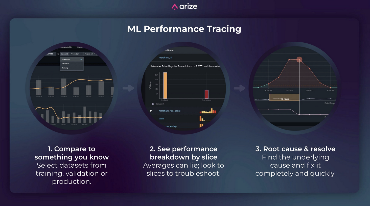
Step 1: Compare to Something You Know
Model performance only really makes sense in relation to something—if the alert fired, something must have changed.
Machine learning models rely on data and code. One of those must be held constant for comparison while you change the other. So you either compare the same model on multiple datasets or multiple models on the same dataset.
Troubleshooting machine learning requires comparing across datasets.
What datasets do we have to compare?
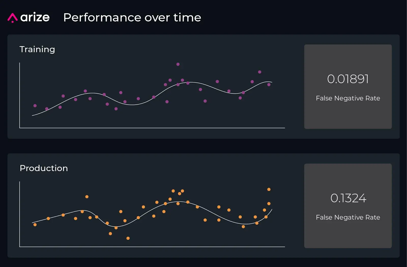
- Training data. Your model must have been trained on something, and you can look for differences between the training dataset and the data you are seeing in production. For example, perhaps a fraud detection model is having an issue in production. You can pull the original training dataset and see how the percent false negative changed since then.
- Validation data. After training your model, you would have evaluated it on a validation dataset to understand how your model performs on data it did not see in training. How does the performance of your model now compare to when you validated it?
- Another window of time in production. If your model was in production last week and the alert did not fire, what changed since then?
You can also compare your model’s performance to a previous model that you had in production. Last month’s model might give you more accurate ETAs for your food delivery, for example.
Step 2: Go Beyond Averages and Analyze Performance of Slices
💡Definition: What Is a Slice?
A dataset slice identifies a subset of your data that may behave qualitatively differently than the rest. For example, rideshare customers picked up from the airport may differ significantly from the “average” riders.
Comparing one metric across the whole dataset is fast, but averages often obscure interesting insights. Most frequently you are looking at a small slice, like a subset of a subset of data. If you can find the right slice, figuring out the problem becomes almost trivial. Ideally, this should not involve hundreds or thousands of SQL queries because you should be able to narrow your options quickly.
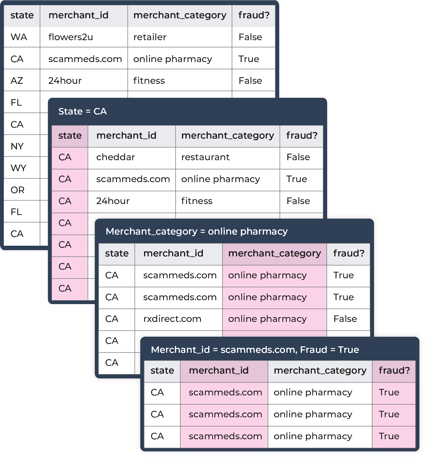
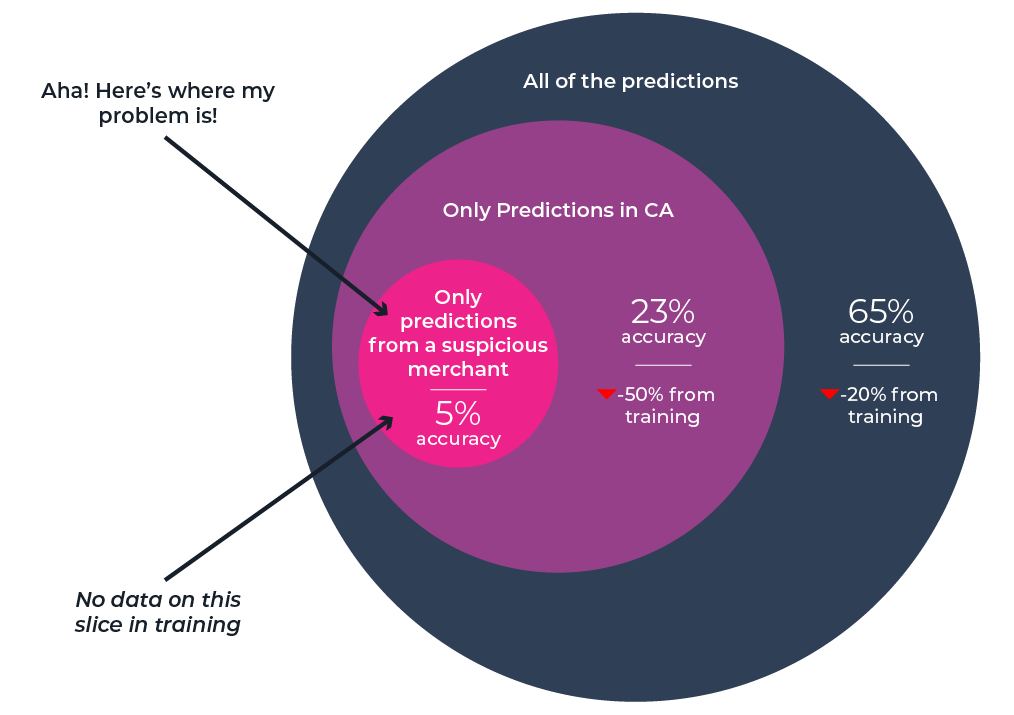
For example, if you saw the entire production dataset for your fraud detection model with slightly abnormal performance, it may not tell you much. If, on the other hand, you saw a smaller slice with significantly worse performance from your California transactions, that may help you identify what’s going on. Better yet: if you narrow it down to California, a particular merchant category, and a particular merchant – and see that all or most transactions were fraudulent –that may help you identify the cause in minutes instead of days.
Real insights often lie several layers down.
You want to be able to quickly identify what is pulling your overall performance down. You want to know how your model is performing across different segments versus your comparison dataset.
This desire is complicated, however, by the exponential explosion in the number of possible combinations of segments. You may have thousands of features with dozens of categories each, and a slice can contain any number of features. So how do you find the ones that matter?
In order to automate this, you need some way to rank which segments are contributing the most to the issue you are seeing. If such a ranking existed, you could employ compute power to crunch through all the possible combinations and sort the amount of contribution from each segment.
Introducing: Performance Impact Score 💡
Performance impact score is a measure of how much worse your metric of interest is on the slice compared to the average.
Ideally, the ML engineer should see where the problem is at a glance. Good visualization and easy navigation can make this process very intuitive and help the engineer focus on providing insight—the job that humans are best at.
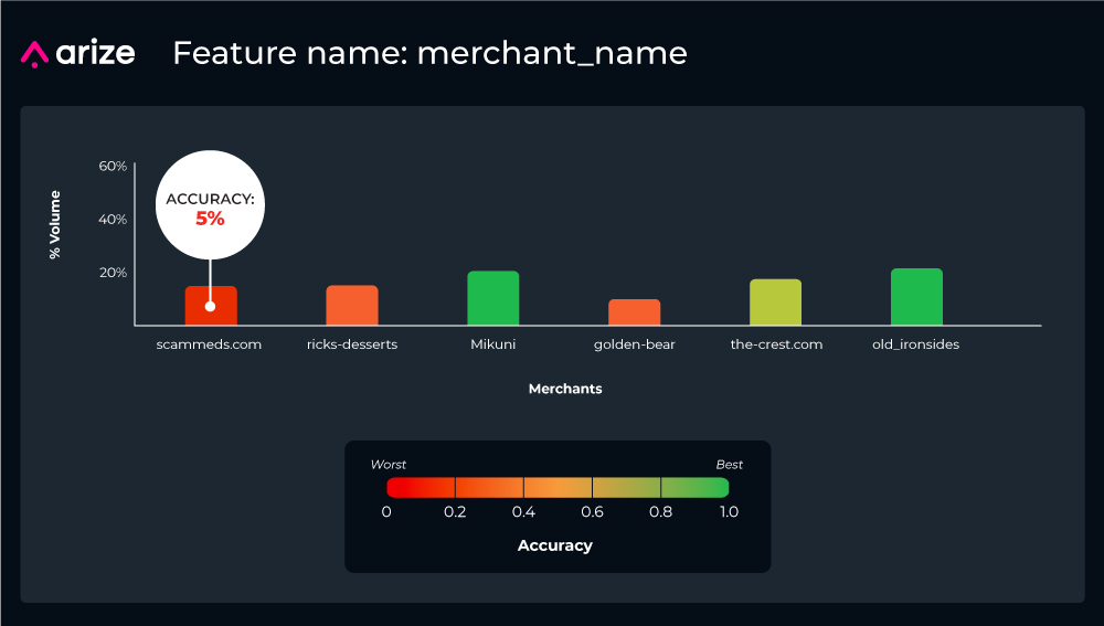
Continuing with the example of the fraud model, sorting by performance impact score enables you to narrow in on a slice – in this case, a specific merchant named “scammeds.com” in California – dragging down performance by 30% compared to the average. Since there was no data for this slice in training, it might indicate the need to retrain the model or revert to a different version.
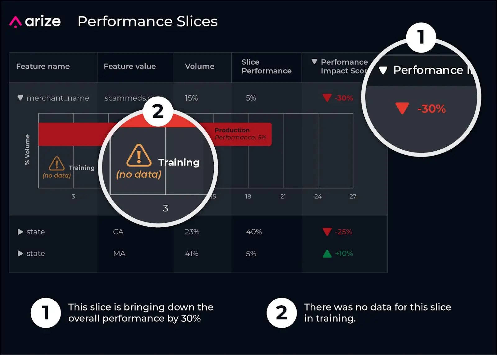
Breaking out the feature “merchant_name” by accuracy and volume further reveals that the model’s accuracy for “scammeds.com” in production is only five percent – hence its drag on overall performance despite only representing a small share of overall transaction volume (~15%).
How Does Explainability Fit Into ML Observability?
Explainability in machine learning refers to the importance of the feature to a prediction. Some features may have much more impact on predicting fraud than others. It is tempting to look at explainability as the holy grail of segmentation, but you must be careful in doing so.
Explainability is the beginning of the journey to resolving the problem, not an end in itself. As Chip Huyen notes, explainability helps you understand the most important factors behind how your model works. Observability, on the other hand, helps you understand your entire system. Observability encompasses explainability and several other concepts.
Using feature importance can help you sort and prioritize where to troubleshoot.
Returning to the example of the fraud model, explainability can be illustrative as to where the problem lies. If you sort by which features have the most importance to the model, you will soon find that the features state (i.e. California) and merchant name (i.e. scammeds.com) are important to examine further to uncover the underlying performance issue.
While explainability is a terrific tool, it should not be used as a silver bullet to troubleshoot your models. Performance impact score offers more information by describing which segment has the biggest impact on why performance dropped.
Step 3: Root Cause & Resolve
You uncovered the needle in the haystack and found where the model is not doing well. Congratulations! Now, let’s get to the harder question—why?
Here are the three most common reasons model performance can drop:
- One or more of the features has a data quality issue;
- One of more of the features has drifted, or is seeing unexpected values in production; or
- There are labeling issues.
Let’s look at those in a bit more detail.
1. One (or more) of the features has a data quality issue
Example: You are trying to figure out why the ETAs for a ride-sharing app are wrong, and you find that the feature “pickup location” is always 0.5 miles off from the actual pickup location.
Recommended solution: The data engineering team needs to go through the lifecycle of the “pickup location” feature and figure out where it gets corrupted. When they find the problem and can implement a feature fix, it should improve the ETAs.
2. One (or more) of the features has drifted, or is seeing unexpected values in production
Example: You see a spike of fraud transactions for your model, but your model is not picking them up. In other words, there is an increase in false negatives. This is coming from a specific merchant ID (which is a feature sent to your model). You are also receiving a huge spike from this merchant ID lately. You should see a drift in this merchant ID feature, showing that you are seeing more transactions from this merchant than before.
Recommended solution: In this case, you want to know what feature has changed either since you built the model or since before the performance decline. You want to find the root cause of the merchant ID distribution drift. After that, you may need to retrain your model, upsampling the new merchant ID that you didn’t see as much of before. In some cases, you might even want to train another model just for this use case.
3. There are labeling issues
Example: A model predicting house prices is showing an extreme discrepancy across price distributions for a particular zip code. Zip code has very high importance. Upon further inspection, you find that the training data reveals this zip code is being labeled with two different city names, such as Valley Village and North Hollywood (the “Hollywood” city name yields higher house prices).
Recommended solution: Highlight the issue to the labeling provider, and provide clarification in labeling documentation.
Conclusion
This post introduces full stack ML observability with ML performance tracing.
To recap: to do ML performance tracing, you must:
- Compare to something you know
- Go beyond averages into slices of data
- Root cause and resolve
Real-life complexities often mean that an error in the smallest slice can lead to a substantial loss of economic value. Today this means that ML engineers must spend a lot of their time writing SQL queries and manually dissecting the model until a solution emerges. There is also a natural tendency to look at explainability as a shortcut. While explainability can often help you understand the problem, it is important to have other tools in your arsenal—particularly performance tracing – to get to the bottom of issues.
Knowing what information to seek and having good tools that surface the information quickly—and in an easily digestible way—can save many hours, dollars, and customer relationships.

